Fall 1996
1. If the expected rate of return on the market portfolio is 12% and DDM Inc. pays a dividend of 4%, by how much must the market believe the stock will increase in price over the next year. You are given the following information on the stock's performance relative to the market portfolio over the last three years.
| Year | Market Return | Return on DDM Inc. stock |
| 1993 | 5% | 3.5% |
| 1994 | 25% | 14% |
2. Tom Jones has $2 million to invest. How much do you think he will put into T-bills, if the yield on his alternative investments are as follows:
| Security | Mean Return | Standard deviation of returns |
| T-bills | 10% | |
| Growth fund | 20% | 35% |
Assuming that the above numbers are in annual terms, how much would Jones put in each of the two securities. You have some information on the kinds of choices that Jones has made in the past in similar situations. Here is what you know:
In 1994, Jones was given the chance to split his investments between a riskless asset paying 7% and a stock index fund expected to yield 15%. The estimated standard deviation of the index fund was 22%. Jones chose to invest $41,000 in the index fund and $59,000 in the riskless asset.
3. If the average correlation between stocks in a basket of risky stocks is 0.2, how many stocks are necessary for effective diversification? You have read in the Financial Analysts Journal that average returns drop by 0.1% for every stock included in a portfolio, due to transactions costs. The average gross return on stocks is 12% per year, and the average standard deviation of returns is 30% per year. You have estimated that your utility function is E(portfolio return) - 0.001 (variance of portfolio returns). Hint: Use Chapter 7, Appendix A. If you cannot get an exact answer, do as much of the computations as you can.
4. Jaeger Corporation stock currently sells for $60 per share. The initial margin requirement is 50% and the maintenance margin is 30%. If Willie Danziger sells short 300 shares of Jaeger stock, to what price can the stock rise before Willie recieves a margin call?
5. a. Compute the expected return and standard deviation of returns for the following stocks:
| Probability | Return on Stock A | Return on Stock B |
| 0.25 | .10 | 0.15 |
| 0.25 | -0.05 | 0 |
| 0.25 | 0.20 | 0.25 |
| 0.25 | 0 | 0.05 |
b. What is the covariance between the returns on Stocks A and B?
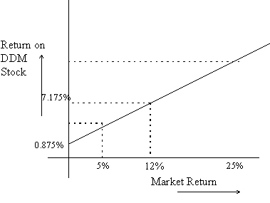
Using the information provided, we can compute the stock's beta to be 0.525. This yields an estimate of the riskfree return of 1,84%, or equivalently, a value of the characteristic line's intercept of 0.875%. Either way, the expected return on DDM stock can be interpolated to be 7.715% when the market return is 12%.
We now use the formula that the rate of return on the stock equals the dividend yield plus the stock appreciation. Hence the stock appreciation equals 7.715% - 4% or 3.715%.
2. From the additional information, we can compute Jones's risk aversion coefficient. We can use the formula for the optimal proportion to invest in the risky asset, from equation 6.3 on p. 181 of the text. This gives us a value of A = 4. We can now compute y* for the data in our problem; y* works out to (20-10)/(.01 x 4 x 352), or .2041 or 20.41% in the risky portfolio, the Growth Fund.
3. From Appendix A (equation 7A.4.), we see that the portfolio variance can be written as 900/n + (1-1/n)(.2)(900) = 180 + 720/n, where n is the number of securities.
Since the expected return is 12 - .1n, the value of the utility function, with n securities is 12 - 0.1n - 0.001 (180+720/n), or 12 - .18 - 0.1n - 0.72/n = 11.72 - 0.1n - 0.72/n
To choose n so that this expression is maximized, we take the first derivative and set it equal to zero. This gives us the equation: 0.1 = 0.72/n2. Solving, we find that n = 2.68. Since we must invest in either 2 or 3 securities, we must compute the utility function for 2 and for 3, to see which is greater. The utility values are 11.49 and 11.61 respectively. Hence the optimal number of securities to invest in is 3.
Alternatively, once the expression for the utility function, 11.72 - 0.1n - 0.72/n , has been obtained, it could be solved simply by trying out different values, and noting the direction of change of the expression for the utility function. Alternatively, we could note from the expression for the variance that as we increase the number of securities from n to n+1, the variance increases by -720/[n(n+1)]. As we increase the number of securities from n to n+1, the expected return increases by -0.1. Hence the value of the utility function increases by -0.1+ 0.001{720/[n(n+1)]} or -0.1 + 0.72/n(n+1). If we start out with 1 security and consider moving to 2, the utility function increases by -0.1 + 0.72/2 = 0.26; hence we would go ahead. If we start with 2 and consider switching to 3, the utility function increases by -0.1 + 0.72/6 = 0.02 > 0; hence we would go ahead. If we switch from 3 to 4, the utility function increases by -0.1 + 0.72/12 < 0; so we would stop at 3.
4. The formula for the actual margin is
Percentage margin = Equity/Value of stock owed.
For our data, we get the equation 0.30 = (27000 - 300P)/300P, since at the beginning, Willie must have put up 300 x 60 x 0.5 in cash plus 300 x 60 from the original sale of the stock = $27000. Solving our equation, we get P = $69.23.
5. The computed numbers are:
| Prob | Ra | Rb | deviation(A) | devn. (B) | prod. of devs. | sq. dev(A) | sq. dev(B) |
| 0.25 | 0.1 | 0.15 | 0.0375 | 0.0375 | 0.001406 | 0.001406 | 0.001406 |
| 0.25 | -0.05 | 0 | -0.1125 | -0.1125 | 0.012656 | 0.012656 | 0.012656 |
| 0.25 | 0.2 | 0.25 | 0.1375 | 0.1375 | 0.018906 | 0.018906 | 0.018906 |
| 0.25 | 0 | 0.05 | -0.0625 | -0.0625 | 0.003906 | 0.003906 | 0.003906 |
| Weighted average | 0.0625 | 0.1125 | 0.009219 | 0.009219 | 0.009219 |
The expected returns are equal to 6.25% and 11.25% respectively for stocks A and B. The variances for both stocks and the covariance between the two stocks all work out to 0.009219. Hence the standard deviations are 9.60% for the two stocks. The correlation coefficient would work out to +1.
1. You have the following obligations and expected cash inflows for the next 5 years:
| Time | In 1 year | In 2 years | In 3 years | In 4 years |
| Obligation | $0 | $10,000 | $20,000 | $1,000 |
| Cash Inflow | $0 | $5,000 | $12,000 |
The following bonds are available at the present time (making annual coupon payments)
| Bond | Maturity | Coupon | Price |
| A | 1 | 0% | 909.09091 |
| B | 2 | 5% | 913.22314 |
| C | 3 | 10% | 1000 |
| D | 4 | 0% | 683.01346 |
a. Construct a portfolio using bonds B and C that immunizes you against parallel changes in the term structure.
b. Construct a portfolio using bonds A and D that immunizes you against parallel changes in the term structure. (15 points for parts a. and b. together)
c. Under what circumstances would these immunized portfolios protect you from interest rate risk? Which immunization plan would better ensure your ability to make your payments as they come due is better? (5 points for part c.)
Bonus: Can you think of a way to shield yourself from interest rate risk in the above situation under any circumstances altogether?
2. a. Using the data from the previous problem what would be your prediction for the yield on three year zero coupon bonds, one year from today, if you knew that the liquidity premium is equal to 1% per year for all maturities. (5 points)
2. b. Assume the following term structure (yields on zero coupon bonds)
| Years | 0.5 | 1.0 | 1.5 | 2.0 | 2.5 |
| Rate | 11.00 | 10.50 | 10.00 | 9.50 | 9.00 |
Two-year bonds that are strippable and paying a coupon of 10.374% are selling at a yield of 10%. Is it worthwhile to strip them and sell the stripped pieces? Or is it better to sell them as a unit? (Assume that you own them and that the strips may be sold at spot yields.) (15 points)
Note: Stripping a coupon bond means selling separately the rights to each of the coupons and to the face value of the bond. Assume that coupons are paid semi-annually.
3. Henrikson ("Market Timing and Mutual Fund Performance: An Empirical Investigation," Journal of Business, v. 54 (1984), pp. 73-96) ran the following regression for 116 mutual funds using data for the period February 1968 to May 1980:
Rpt - Rft = ap + bp(Rmt - Rft) - cp Zt + ept, where
Zt = 0 if Rmt is greater than or equal to Rft
= Rmt - Rft otherwise.
He obtained the following results:
| Period | Feb. 1968 to June 1980 | May 1974 to June 1980 |
| Average estimate of | ||
| ap | 0.0007 | 0.0022 |
| bp | 0.92 | 0.86 |
| cp | -0.07 | -0.08 |
| Number of funds with statistically significant (at 95% confidence levels) | ||
| ap > 0 | 11 | 21 |
| ap < 0 | 8 | 5 |
| cp > 0 | 3 | 2 |
| cp < 0 | 9 | 3 |
What do these results tell you about:
a. the market timing ability of these managers (10 points)
b. the ability of these managers to pick undervalued and
overvalued stocks. (10 points)
4. How does an index model in the construction of an optimal portfolio? Give one advantage and one disadvantage of moving from a single index model to a multi-index model. (20 points) (Hint: Consider the conditions under which the single-index model is valid. You should be able to answer this question using the material in Chapter 9, even though the multi-index model is not explicitly discussed in that chapter.)
5. Is it always better for older investors to invest in risky securities than in less risky securities? Comment on two different aspects:
a. the inherent riskiness of assets for investors with different time horizons. (10 points)
b. the relevance of human capital for investors with different time horizons. (10 points)
Explain your answers in parts a. and b. with examples.
1. It is easy to ascertain that the yields on bonds A, B, and C are all 10%. Hence the term structure must be flat at 10%. Using this information, the duration of the net obligations of the individual works out to 2.68. The present value of the net obligations equals $10,825.80.
| Year | 1 | 2 | 3 | 4 |
| Outflow | (10,000.00) | $(20,000.00) | $(1,000.00) | |
| Inflow | $ 5,000.00 | $ 12,000.00 | ||
| Net flow | $0 | ($5,000) | ($8,000) | ($1,000) |
| PV | 0 | -4132.2314 | -6010.51841 | -683.01346 |
| [PV/Sum(PV)]xYear | 0 | 0.76340694 | 1.66561514 | 0.2523659 |
The durations of the bonds can be worked out more easily; for bonds A and D, the duration equals the maturity, for bond C, which is selling at par, rule 8 can be used; for bond B, rule 7 can be used.
| Bond | Maturity | coupon | Price | Duration |
| A | 1 | 0% | 909.090909 | 1 |
| B | 2 | 5% | 913.22314 | 1.95 |
| C | 3 | 10% | 1000 | 2.74 |
| D | 4 | 0% | 683.013455 | 4 |
We need to create portfolios with durations equal to 2.68. Since the yields of all the bonds are the same, the duration of any portfolio is equal to the value-weighted average of the individual bonds. Hence, we can construct the required portfolio of bonds A and D by buying $10,825.80 worth of bonds, with x% of the portfolio invested in bond A, and the remainder in bond D, where 1x + 4(1-x) = 2.68; solving, x works out to 0.44.
Similarly, we can invest the same amount in bonds B and C with y percent in bond B and (1-y) percent in bond C, where 1.95y + 2.74(1-y) = 2.68. Solving, we get y = 7.59%.
The immunization plan would only work for small and parallel changes in the yield curve. Furthermore, the portfolio consisting of bonds A and D would be better because the cash flows would be dispersed. (Effectively, this provides greater convexity for the asset portfolio, than for the portfolio of obligations.) However, it would be possible to shield against interest rate risk completely by constructing a portfolio using bonds A, B, C, and D so that the net flows in each period from the portfolio equal the net obligations in that period. This can be done by solving a system of four linear equations.
2. a. Since the yield curve is flat at 10%, all forward rates equal 10%. We know that the long yield is the average of the short rate and the forward rates. The expected short rate next period is equal to the forward rate less the liquidity premium, i.e. 10% - 1% = 9%. The forward rates next year should all be 10% again. Hence the expected yield one year hence, on three year zero coupon bonds equals, approximately, (9+10+10)/3 = 9.67%.
2. b. The coupons from the 2 year bond would be $10.374/2 = 5.187 every six months for 2 years, plus $100 at the end of 2 years. Pricing the bond, using the given yield of 10% gets us $100.664. However, computing the present value of the strip cash flows separately at the given term structure yields and adding them up gets us 101.94. Hence stripping the bond and selling the pieces is better.
| Years | 0.5 | 1 | 1.5 | 2 |
| Rate | 11 | 10.5 | 10 | 9.5 |
| Strip Cash Flow | 5.187 | 5.187 | 5.187 | 105.187 |
| PV | 4.92 | 4.68 | 4.48 | 87.36 |
3. For the two time periods respectively, 9.5% and 18% of the fund managers were able to pick mispriced stocks, as can be seen from the first row of the second part of the table. On the other hand, 6.9% and 4.3% respectively of fund managers underperformed in the two periods. There seems to be little, if any, evidence overall of fund managers being able to recognize mispriced stocks.
Given that 3 and 2 managers display positive timing ability (third row of second part of table) and 9 and 3 managers display negative timing ability (for the two time periods respectively), there is absolutely no evidence in this table that fund managers can time the market.
4. The advantage is that by increasing the number of factors, we can ensure that the residual from the regression truly measures unsystematic risk. If there were industry or other factors (other than the market index factor in a single index model), the resulting risk estimates would be biased downwards. On the other hand, computation would be more difficult, and we would have greater estimation risk.
5. The appendices to chapter 7 make it clear that there is no reason for older and younger investors to pick different portfolios from the point of view of the inherent riskiness of the assets.
However, if an investor has human capital with low risk, it might make sense for such a person to invest a greater amount of his/her non-human capital in a high risk portfolio when young, and to switch money into less risky assets as time went by and the market value of the human capital decreased.
On the other hand, if a person were working in the mutual fund industry, it may be argued that his/her human capital is highly risky, and it may be optimal for him/her to invest in relatively riskfree assets during the early part of his/her life.