Estimation of Discount Rates
©Prof.
P.V. Viswanath, 1997
- Term Structure of Riskless Interest Rates
- Term Structure of Risky Interest Rates
- The riskfree rate
- The market risk premium
- Beta Estimation
- Weighted Average Cost of Capital
Term Structure of Riskless Interest Rates
There is a term structure of riskless interest rates. In other words, the annualized rate of interest is not necessarily the same for one year loans, two year loans, three year loans, etc.
Why should these rates differ? The simplest way to understand this is to realize that when a lender lends for more than one year, say, for two years, s/he is lending for the first year and simultaneously making a commitment to lend for the second year at a prespecified rate of interest. Instead of doing this, he could lend for one year at a time. If he did this, he might end up better off if rates the second year turned out to be higher. But then, the borrower would be worse off, ex post. Or he might be worse off; and the borrower would turn out to be better off. Either way, there is no reason to believe that the borrower or the lender would be indifferent about making a commitment to borrow or lend one year ahead at a prespecified interest rate. Depending upon expectations about what might happen to interest rates in the future, annualized interest rates on two year loans might be higher (if rates were expected to go up in the future) or lower (if rates were expected to drop in the future) than annualized interest rates on one year loans.
Term Structure of Risky Interest Rates
Similarly, there is also a term structure of risky interest rates. Let's see why this is relevant. Suppose we have a project with cashflows of $20 in year 1, $100 in year 2 and $150 in year 3. What is the present value of this project? To begin with, we can write:
PV(0,20,100,15) = PV(0,20,0,0) + PV(0,0,100,0) + PV(0,0,0,150)
That is, the present value of the project is equal to the sum of the present values of the three different cash flows. If we let CFi stand for the cashflow in year 1, and ri stand for the annualized discount rate appropriate to that cash flow, then we have,
PV(CFi) = CFi/(1+ri)i
For example:
PV(0,0,100,0) = 100/(1+r2)2
where r2 is the required rate of return appropriate for cash flows of the given riskiness generated in 2 years from now.
If we go with the CAPM, and we assume that the beta risk of that cash flow equals b, then we know that
r2 = rf + b(Mkt. risk premium)
There are three different quantities to be estimated here.
- the risk free rate
- the beta
- the market risk premium
Normally, we use the yield on fixed income Government securities, i.e the yield on a Government security that pays $1 at the appropriate time in the future. Thus, if wish to obtain the value of r2, the required rate of return on risky assets paying out cash flows only at time 2, we would use for rf, the yield on a zero-coupon T-bond with a maturity of 2 years.
Unfortunately, zero-coupon T-bonds do not exist for all the desired maturities. We can, therefore, take the yield on a T-bond with an approximate effective maturity (called duration, see books on Investments) equal to the desired maturity. In principle, then, we should be using a different riskfree rate for different years. In practice, a single rate is used, for convenience. We could try two different methods, using a short-term rate, say a 3-month T-bill rate, and a long-term rate, say the rate on 30 yr. T-bonds, and perform some sensitivity analysis before going in for more precision in the discount rates.
The approach taken here is a two-fold one. First, use a historical estimate; second, adjust this historical estimate for differences between the current economic situation and the average historical situation. How do we come up with a historical estimate. We must first decide which riskfree rate to use. Once we have decided on that, we compute the realized risk premium for each year in some not too distant period in the past (say, the last 25 years). This realized risk premium is simply the ex-post return on the market portfolio less the riskfree rate.
Now, we take the average of this time series. Here we again come up with the question of how distant the cashflow is, and the term structure of risky interest rates. Keep in mind that what we want is a rate that we will be using to compound. In other words, even though we may write the present value of CF3 as CF3/(1+r3)3, what we really want is CF3/(1+cr3), where cr3 is the compounded required rate of return on a security of the appropriate beta risk with a single cashflow three years from now.
Now, if we have a data series on realized returns on such a security for the last twenty years, how would we come up with an estimate of cr3? Obviously, we really only have one observation, since we only have one 3 year period before us. The requisite estimate, therefore, is simply the actual compounded return over those twenty years. Now, this means that if we wanted a estimate of r3, the annualized rate, we would take the gross compounded 3 year return (1+cr3) and take the third root, and subtract one, so that when we compound it, we get the right value. For example, suppose the actual return on the a security with similar beta risk had been 20%, -10%, and 50% over the last three years. Then, an investment of $1 three years ago, would have grown to $1.20 the following year, dropped to 0.9(1.2) or 1.08, the year after that, and then grown to 1.62 for a compounded return of 62% over the three years. If we wanted to annualize it, we would take the third root of 1.62 and subtract one to get 17.446%, so that when we computed (1.17446)3, we would get back 1.62, as required.
What we have, in effect, done is to take the geometric average of the data series. On the other hand, if we wanted an estimate of the return on this same security over a 1 year period, what we would do is to take the simple average or arithmetic mean, which turns out to be 20%, which is greater than the geometric mean. We don't compound this, since what we want is the return for one year and not for a greater number of years.
What do we do if we wanted cr3, but had a larger data series? One way would be to compute three year compounded returns and then compute the simple average of those compounded returns. Again, this would be the correct approach in principle, but just as in the case of the riskfree rate, a more practical approach is simply to take the geometric mean or the arithmetic mean. In general, we might go with the geometric mean, the longer the period is, and with the arithmetic mean, the shorter the period is. The same reasoning is applied in the case of the market risk premium. For projects with cashflows mainly out in the future, we might use the geometric mean of our realized risk premium series to estimate the future market risk premium, while we would use the arithmetic mean of the realized risk premium series to estimate the future market risk premium if the cash flows were not too distant. We would also use the short term T-bill rate in the latter case to generate the realized risk premium series, and the long-term T-bond rate in the former case.
Now that we have our historical estimate, we must look at the factors determining the market risk premium. These are, briefly,
- Uncertainty in the Underlying Economy
- Political Risk
- Structure of the Market
An alternative to using a historical market risk premium estimate is to use the implied risk premium. This can be computed using Damodaran's Excel template, slightly modified by me.
Evidence that the term structure of equity risk premiums is not flat and an estimation methodology has been presented by J. Benson Durham of the NY Federal Reserve Bank. More on this can be found on the NY Fed's website.
Again, we use a combination of the historical and fundamental approaches. The historical estimate requires a regression of the realized stock returns on the company's stock on the realized market stock returns. Some issues to be taken into account here are:
- Length of the Estimation period
- Return Interval
- Choice of Market Index
- Adjustment of estimated beta
Determinants of beta
- Cyclical Nature of business
The greater the cyclicity of revenues from an asset, the higher its beta. - Degree of Financial Leverage
- Degree of Operating Leverage
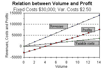
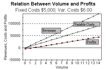
Consider these two technologies which can be used to manufacture a product selling for $10/unit.

When fixed costs are higher and variable costs are lower, profits are more responsive to changes in volume. If volume is highly correlated with the market, then this translates to higher asset betas.
You can also access an Excel file containing the data used to generate these two figures. (Click here for information on how to download Excel files.)
The fundamental approach may have to be resorted to if historical data on the stock returns of the company are not available. In this case, we may also use the betas of firms in comparable industries, and do the appropriate deleveraging and leveraging as necessary to adjust for differences in financial leverage.
Weighted Average Cost of Capital
Although in principle, the entire approach detailed above can be used for the project directly, in practice, a cost of capital (or required rate of return) is computed for the entire firm. Then, an assumption is made that the project under consideration is similar to the entire firm. The approach detailed above is then applied to compute the required rate of return on the common stock of the firm. Other approaches are used to compute the required rates of return on the other liabilities of the firm. The cost of capital of the entire firm is then the weighted average of the estimated required rates of return on the different securities issued by the firm, where the weights are the market value shares of the different security classes. The security classes that have to be taken into account are:
- Common Stock
- Bonds
- Preferred Stock
- Convertible Stock