All bonds are subject to Capital Gain Risk, if the maturity of the bond differs from the bondholder's horizon.
Suppose the market interest rate drops to 7.8%. The market price is
now given by 50![]() + 1000/(1.039)4
= 1040.02.
+ 1000/(1.039)4
= 1040.02.
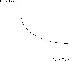
As the bond yield drops, the bond price rises, and vice-versa.
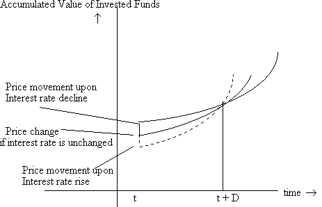
Scenario 1: The interest rate drops to 7.8%, soon after the bond is purchased, and stays there. The bond price rises immediately to 1040.02. After six months, the bond price rises to 1040.02 (1.039) = 1080.58. At this time, a coupon of $50 is paid, whereupon the price of the bond drops by an equal amount to 1030.58. The bond increases in value at the end of the year to 1030.58 (1.039) = 1070.77, while the $50 coupon is reinvested at an annual yield of 7.8% and grows to 50 (1.039) = 51.95, for a total of 1122.72.
Scenario 2: The interest rate rises to 8.2%, and stays there. The price
immediately drops to 50 ![]() + 1000/(1.041)4 = 1032.59. However, the bond and coupons thereafter rise
at the rate of 4.1% every six month, culiminating in a value of 1119.00
at the end of the investment horizon.
+ 1000/(1.041)4 = 1032.59. However, the bond and coupons thereafter rise
at the rate of 4.1% every six month, culiminating in a value of 1119.00
at the end of the investment horizon.
What we see is that if interest rates drop and stay there, there is an immediate appreciation in the value of the portfolio, but the portfolio then grows at a slower rate; on the other hand, if interest rates rise and stay there, there is a capital loss, but the portfolio then appreciates more rapidly. Hence there is some investment horizon, such that investors with that horizon, will not care if interest rates drop or rise (as long as the changes are small). This horizon is shown in the figure below as D. We will see below that the value of D depends on the characteristics of the bond portfolio; specifically, we will see that D is simply the duration of the bond portfolio.
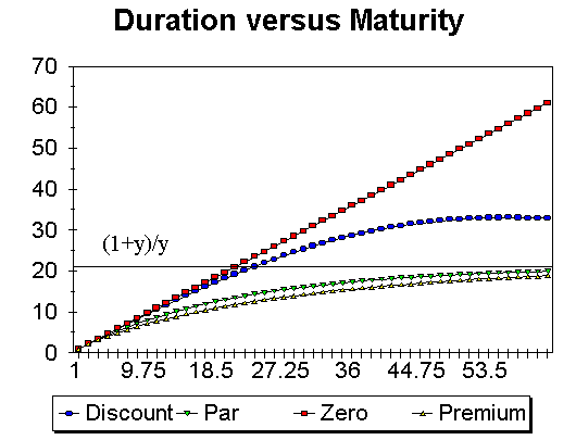
A stock's risk is measured by its beta, which looks at the stock's sensitivity to market movements. The same thing could be done, in principle, with bonds. However, there are two further issues: one, interest rates are the main source of risk for bonds; two, obtaining return data on bonds to measure a market beta is difficult because a) bonds are often not traded; and b) the maturity of a bond changes with time, and hence its identity. Consequently, bond price risk is, most often, measured in terms of the bond's Interest Rate Sensitivity.
Bond pricing formula where y is the yield and Ci, the cash flow in period i:
![]()
Assuming that the yield curve moves parallel to the initial yield curve, we can differentiate with respect to the yield, y, to obtain:
![]() , where D is the Macaulay
duration and is defined as:
, where D is the Macaulay
duration and is defined as:
![]() , where
, where
present values are computed using the yield to maturity, y.
Consider a 2 year, 10% coupon bond selling at par. In this case, the
case flows are as follows:
| Time | 0.5 | 1 | 1.5 | 2 |
| Cash flow | 50 | 50 | 50 | 1050 |
| PV/Price | 0.0476 | 0.04535 | 0.04319 | 0.8638 |
| (PV/Price)xTime | 0.0238 | 0.04535 | 0.064785 | 1.7277 |
Modified Duration = Macaulay Duration/(1+y)
Hence, Modified Duration x P = delta(P)/delta(y)

where dy is the yield change, and dP is the price change.
Example:
We computed the duration of a 2 year, 10% coupon bond selling at par
as 1.8616 years or 3.7232 half-years. For this bond, if the yield changes
from 5% per 6 months to 4.5%, the price change can be estimated to be [-3.7232
x 100/1.05] 0.005 = $1.77, whereas the actual price change is given by
100 - [5 ![]() + 100/(1.045)4], or $1.79.
+ 100/(1.045)4], or $1.79.
This formula only works for small yield changes, because the price of a bond as a function of yield is nonlinear. In other words, the duration of a bond changes as the yield changes. The price approximation is improved if we can take into account this nonlinearity. This is what is known as convexity.
Convexity is defined as (d2P/dy2)(1/P), and can
be computed as  .
.
For bonds with a constant coupon of $C per period, there is a closed-form
solution for the second derivative: 
Note: Convexity in years = Convexity in m periods per year/m2, while Duration in years = Duration in m periods per year/m.
dP/P = -D* (dy) + 0.5 (Convexity) (dy)2
For a 6%, 25-year bond selling to yield 9%, the modified duration works out to 10.62 years, while the convexity is 182.92 (in years). The estimated percentage price change, for a yield change from 9% to 11% is -10.62 (0.02) +0.5 (182.92) (0.02)2 = -21.24 + 3.66% = -17.58%, while the actual change is -18.03%.
If the yield decreases by 200 basis points, instead, then the estimated price change is +21.24% due to duration, and +3.66 due to convexity, or 24.90%; the actual price change is 25.46%. The estimated price change is no longer symmetric about the current yield, because the price function has curvature.
Example: Compute the convexity for an 5 yr., 8% bond selling at par.
We use the formula  .
.
| Period | Cash Flow | |
| 1 | 4 | 7.1119709 |
| 2 | 4 | 20.515301 |
| 3 | 4 | 39.452501 |
| 4 | 4 | 63.225162 |
| 5 | 4 | 91.190138 |
| 6 | 4 | 122.75595 |
| 7 | 4 | 157.37943 |
| 8 | 4 | 194.56248 |
| 9 | 4 | 233.84914 |
| 10 | 104 | 7145.3902 |
| Sum | 8075.4323 |
convexity in half years (d2P/dy2)(1/P) = 8075.43/100 = 80.7543
Convexity in years = 80.7543/4 = 20.1885
Dollar convexity = Price x convexity = 100 x 20.1885 = 2,018.85
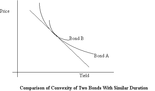
Bond B has greater convexity than Bond A. Whether the yield rises or falls, Bond B will have a higher price. Hence, while it may happen at times that two bonds of different convexities will be priced similarly, as in the figure above, normally convexity will be priced. Ceteris paribus, bond B will command a higher price than bond A.
How much should the market want investors to pay up for convexity? If investors expect that yields will not change much, then there is not much of an advantage to higher convexity, while if yields are expected to change a lot, convexity will be highly valued. In general, investors with higher than average volatility expectations will be willing to pay for buy convexity (buy the higher convexity bond and sell the lower convexity bond), while investors with lower than average volatility expectations would be willing to sell convexity.
Over the 1930-1979 period, the following was found to be true:
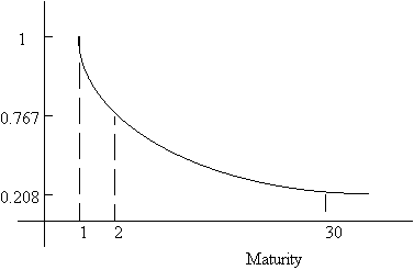
Average Change in YTM as a multiple of the change in YTM for 1 year bonds.
That is, long term rates are less volatile than short term rates. Immunization must therefore take this into account. More complex formulas have been computed allowing for particular kinds of non-parallel shifts in the yield curve, but this added complexity does not seem to have paid off in more effective immunization. Work currently under way models the term structure as composed of two (or more) stochastic factors. It is then possible to write the future value of any portfolio in terms of its exposure to the two (or more) factors. Under these circumstances, immunization would imply equating the sensitivities of asset and liability portfolios to the stochastic factors.
Portfolio I, referred to as the 'bullet' portfolio consists of Bond C.
Portfolio II, called the barbell portfolio, consists of 50.2% of bond
A and 49.8% of bond B.
| Bond | Coupon | Maturity (yrs.) | Price plus Accrued | Yield | Dollar Duration | Dollar Convexity |
| A | 8.50 | 5 | 100 | 8.50 | 4.00544 | 19.8164 |
| B | 9.50 | 20 | 100 | 9.50 | 8.88151 | 124.1702 |
| C | 9.25 | 10 | 100 | 9.25 | 6.43409 | 55.4506 |
The convexity of the two portfolios differs: The bullet portfolio has a dollar convexity of 55.4506, while that of the barbell portfolio is 71.7846. (Note that consistent with the higher convexity of the barbell portfolio, it has a higher price, i.e. a lower yield. This yield can be computed as a weighted average of the yields of the two bonds making up the portfolio, and it works out to 8.998%.)
Given the similar durations of the two portolios, the bullet and barbell portfolios will perform similarly for small changes in yield (if the yield curve changes in parallel). However, for larger changes, since the barbell portfolio has larger convexity, it will do relatively better than the bullet portfolio.
However, we cannot make similar claims if the yield curve changes in a non-parallel fashion. When the yield curve flattens, the barbell portfolio dominates the bullet portfolio, while for a steeper yield curve, the barbell is better, for large drops or large rises in the yield, but worse otherwise.
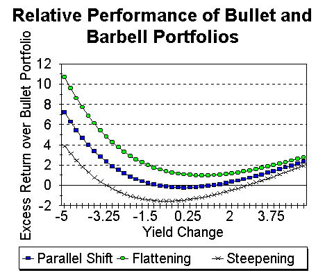
| Yield Change | Parallel Shift | Flattening | Steepening |
| -5 | 7.19 | 10.68 | 3.88 |
| -4 | 3.99 | 6.88 | 1.27 |
| -3 | 1.88 | 4.25 | -0.37 |
| -2 | 0.59 | 2.55 | -1.25 |
| -1 | -0.07 | 1.54 | -1.57 |
| 0 | -0.25 | 1.06 | -1.48 |
| 1 | -0.09 | 0.98 | -1.09 |
| 2 | 0.31 | 1.18 | -0.49 |
| 3 | 0.89 | 1.58 | 0.24 |
| 4 | 1.57 | 2.12 | 1.06 |
| 5 | 2.31 | 2.75 | 1.92 |
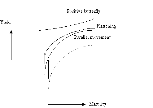
Butterfly changes account for about 3.4% of Treasury returns, while parallel shifts and twists account for 91.6%, with 5% unknown. (Frank Jones, "Yield Curve Strategies," Journal of Fixed Income, Sept. 1991, pp. 43-48.)
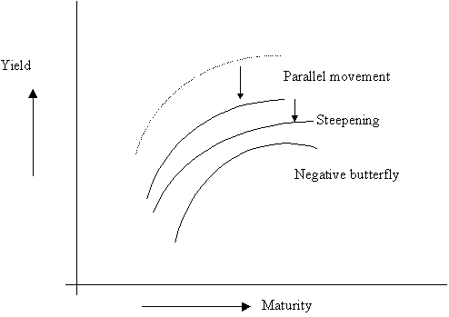
Empirically, an upward shift and flattening of the yield curve is accompanied by a positive butterfly movement (less humped), while a downward shift and a steepening of the yield curve is correlated with a negative butterfly movement.
The following strategies have been shown to work will under the following
different scenarios.
| Yield Decreases | Yield Increases | |
| SteeperYield Curve | Intermediate Maturity
Bullet |
Short Maturity
Bullet |
| Flatter Yield Curve | Long Maturity Barbell (around long maturity) |
Short or Long Maturity
(greater flattening relative to upward yield shift favors the long maturity) |
A positive butterfly movement implies that yields on intermediate maturity bonds drop in price and hence a movement towards an intermediate maturity is warranted.
The idea is to create a portfolio that mirrors the composition of an index that measures the broad market (e.g. the S&P 500 Index is used for equity index funds).
Bond Indexes:
There are three major bond indexes of the broad bond market: the Salomon Brothers Broad Investment Grade (BIG), the Lehman Brothers Aggregate Index, and the Merrill Lynch Domestic Master Index. All three indexes inlcude bonds with maturities greater than one year; as the maturity of a bond falls below a year, it is dropped from the index.
Considerations in choosing an index:
There are several problems with tracking a bond index:
c) maturity; d) market sectors (Treasury, corporate, mortgage-backed, etc.); e) credit rating; f) call factors; and g) sinking fund features.
The objective is then to select from all of the issues in the index, one or more issues in each cell that can be used to represent the entire cell. The total dollar amount invested in each cell will depend upon the share of that cell in the entire universe of securities represented in the index. The number of cells used will depend on the dollar amount of the portfolio to be indexed. A portfolio with a small dollar value will have fewer cells, so as not to increase tracking error due to transactions costs.
The Optimization approach is also a cellular one; however, the choice of securities from each cell is made with a view to achieving some other objective, such as e.g. maximizing yield to maturity, maximizing convexity, etc; Mathematical programming is used to achieve this goal.
The Variance Minimization approach uses historical data to estimate the variance of the tracking error for each issue in the index, and then use that to minimize the total variance of the tracking error. The tracking error variance of a given security is obtained by estimating the price function for that security as a function of its cash flows, duration, and other sector characteristics. Quadratic programming is then used to find the optimal index portfolio in terms of minimized tracking error. Since it is difficult to get enough data on each security, this approach is very difficult.
Net Worth = PV(A) - PV(L) = [-DAPV(A) + DLPV(L)]y/(1+y), which is not equal to zero, where Di , i = A, L stands for the duration of the assets and the liabilities respectively. Hence equating durations will work only if PV(A) = PV(L). In general the condition that must be satisfied is:
DAPV(A) = DLPV(L)
If we define immunization as a strategy that ensures that the terminal value is not smaller than the initial value, then we can write the necessary conditions as:
Duration(assets) = Duration(liabilities)
PV(Assets) greater than or equal to PV(Liabilities)
There are additional complexities if there are multiple liabilities, as is usually the case. This is dealt with later. In addition, Gap Managers may also be interested in keeping the ratio of Net Worth to Assets or some other measure immunized with respect to interest rate changes.
It is worthwhile at this point to revisit the twin effects of a yield change.
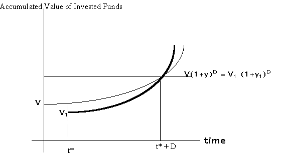
Consider a portfolio with a value of V at time t*-![]() (the instant before t*). If the yield on the portfolio is y, the portfolio
value will increase at the rate y. Let D be the duration of the portfolio.
At time t* + D, the value of the portfolio is V(1+y)D. Now suppose the
yield increases at time t*, so that the portfolio value drops to V1.
However, because of the higher yield, the portfolio value increases at
the higher rate y1. In how many periods, will the portfolio
value reach V(1+y)D? It can be shown that this happens in exactly D periods.
(the instant before t*). If the yield on the portfolio is y, the portfolio
value will increase at the rate y. Let D be the duration of the portfolio.
At time t* + D, the value of the portfolio is V(1+y)D. Now suppose the
yield increases at time t*, so that the portfolio value drops to V1.
However, because of the higher yield, the portfolio value increases at
the higher rate y1. In how many periods, will the portfolio
value reach V(1+y)D? It can be shown that this happens in exactly D periods.
That is, V(1+y)D = V1(1+y1)D
In other words, as explained earlier in the webnote, the duration of a portfolio is exactly the amount of time that it takes for the change in value due to a yield increase to be made up by the increased reinvestment rate. This also makes it clear that if an insurer desires to have a certain amount of money, say $10,000 available for payouts in k years, and the discounted present value of those $10,000 is available today (i.e. the liability if fully funded), then those funds must be invested in a portfolio with a duration of k years. In this way, the portfolio is immunized against changes in value for small changes in the yield. Alternatively, the duration of the asset portfolio must match that of the liability portfolio.
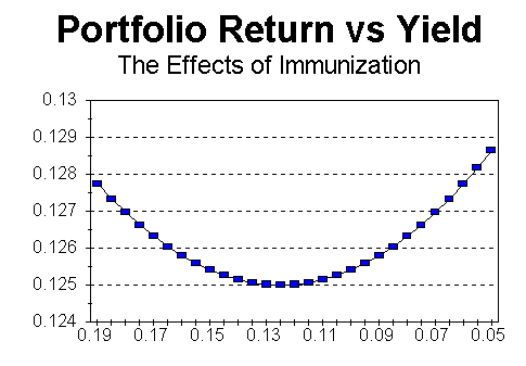
We have below a graph of portfolio value as a function of yield, assuming that there is one yield change immediately, and none thereafter:
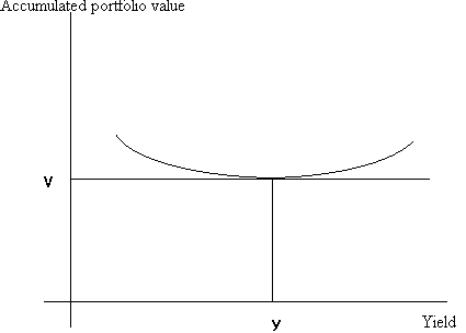
Note that the accumulate portfolio value remains at V for very small changes in y. However, for larger changes in y, the portfolio value increases, both for yield increases and for yield decreases. (This is due to bond convexity.)
Example:
Consider an insurance company with a single liability of 17,183,033 in exactly 5.5 years. Suppose the company purchases an 8-year, 10.125% bond selling to yield 12.5%. Assume coupons can be reinvested at this rate.
In order to fund the liability fully, the company would need to purchase
bonds worth 17,183,033/(1.0625)11 = 8,820,062.20. The price of an 8-year
10.125% bond selling to yield 12.5% can be computed to be ![]() = 9.9346(5.0625) + 51.33 = 88.20262; hence the face value of the bonds
purchased is 8,820,062.20/88.20262 = $10 m. Suppose the yield changes to
12%. In this case, the value of the portfolio would rise to
= 9.9346(5.0625) + 51.33 = 88.20262; hence the face value of the bonds
purchased is 8,820,062.20/88.20262 = $10 m. Suppose the yield changes to
12%. In this case, the value of the portfolio would rise to ![]() = 5,116,109.5 + 3,936,462.8 = 9,052,572. This would grow to 9052572(1.06)11
= 17184484 at the end of 5.5 years for a gain of $1451. It can be confirmed
that the value of the portfolio would be greater than the target 17183033
for any yield change at all.
= 5,116,109.5 + 3,936,462.8 = 9,052,572. This would grow to 9052572(1.06)11
= 17184484 at the end of 5.5 years for a gain of $1451. It can be confirmed
that the value of the portfolio would be greater than the target 17183033
for any yield change at all.
Note that the duration of the 8-year 10.125% bond selling at a price of 88.20 is exactly 5.5 years.
The way this additional condition works can be illustrated graphically as follows:
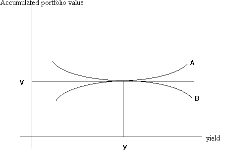
Both portfolios A and B satisfy the duration condition: the value of both portfolios remain constant for very small changes in yield. However, for larger changes in yield, portfolio B will lose value, and will not be immunized.
Mathematically, dispersion is given by the following formula:
 , where
CFi is the cash flow at time i, and D is the duration of the bond portfolio.
Rebalancing in an immunization strategy
The duration of a single period liability will change at the rate of 1 per year, while that of the asset portfolio will not necessarily change so smoothly. This also applies to multi-period liabilities. (Durations will decrease smoothly until a coupon payment is made.) Hence, it will be necessary to rebalance the asset portfolio to maintain the equality of durations, even if yields do not change.
Cash flow matching and dedication
Cash flow matching implies constructing an asset portfolio that has cash flows that are equal in magnitude and opposite in sign to the obligation. In a multiperiod context, cash flow matching is called dedication.
The following graph shows how duration is affected when bonds are combined into portfolios.
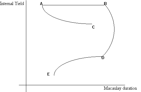
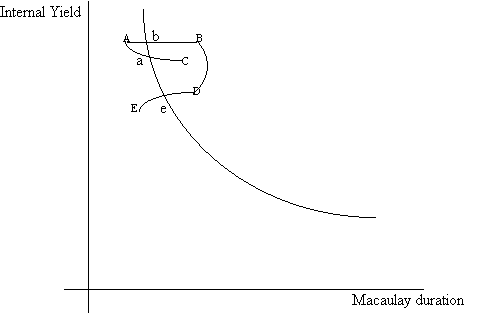
Climbing The Immunization Curve
Consider a given liability portfolio. It's duration depends on the rate used to discount the portfolio's cash flows. The 'immunization curve' relates duration to yield. Suppose there are four assets, A, B, D, and E. We need to find a portfolio of these four assets with the same duration as our liability. IF we discount the liability portfolio using the yield on the portfolio of assets, we can see that there are several such portfolios--a, b, and e. Since portfolio b has the highest yield, we would prefer that portfolio, so that we can minimize the total investment required for immunization.
Of course, this procedure makes the strong assumption that the yield curve is flat at the yield level of the asset portfolio; hence one must be careful not to rely too heavily on this technique.
For example, if it is expected that the yield curve will remain fairly constant over time, then holding higher maturity bonds may be preferred to holding shorter maturity bonds. In this way, the bonds can be purchased at a high yield (low price) and then sold at a low yield (high price).
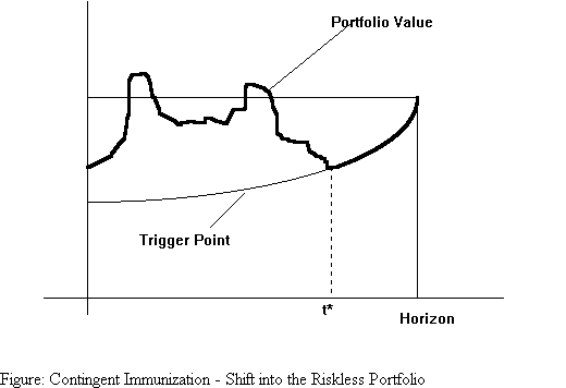
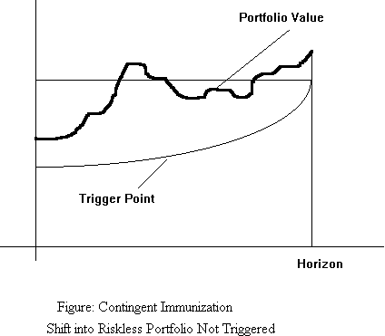
A portfolio manager may have a minimum portfolio value in mind at a prespecified horizon point. He has two alternatives: one, to put the available money in a fully immunized portfolio that is guaranteed to attain the required minimum portfolio value at the horizon point. Alternatively, if he currently has a greater sum of money that is required in order to attain that minimum value, he may choose to invest it in a riskier portfolio, switching to the riskless strategy whenever his portfolio value drops to the level at which a riskless strategy will yield exactly the desired minimum portfolio value at the horizon point. Such a strategy may result in a switch to the riskless portfolio, at some time t*, as shown in the diagram below, or, if the manager's strategy is sufficiently successful, he may never have to switch to the riskless portfolio as in the second diagram.
The expected yield to maturity can be computed as the weighted average of all possible yields, weighted by their probabilities.
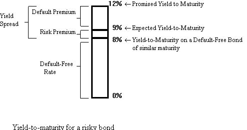
To compensate investors for the possibility of bankruptcy, a corporate bond must offer a default premium. This default premium is a differential in promised yield between the corporate bond and its expected yield to maturity.
The default premium depends on two main factors:
d = y - ![]() (where
y is the promised yield-to-maturity, and
(where
y is the promised yield-to-maturity, and ![]() is the expected yield to maturity), can be given by:
is the expected yield to maturity), can be given by:
![]()
Example:
Suppose Bond A has a promised yield-to-maturity of 12%, but owing to a high default risk, the expected yield is only 9%.
Assume that this bond has a 6% annual default probability and that it is estimated that if the bond does default, each bondholder willl receive an amount equal to 60% of the bond's market price a year earlier. What is the equilibrium default premium on this bond?
Using the above formula, the default premium of the bond should be
(.09 + 0.4x.06)/0.94 - .09 = 0.0313, or 3.13%. In other words, the promised yield should be 12.13%, which is relatively close to the 12%, assumed in the example.
The riskiness of individual bonds depends on various factors, such as:
| Moody's | S&P |
| Investment Grade Bonds | |
| Aaa | AAA |
| Aa | AA |
| A | A |
| Baa | BBB |
| Speculative Grade Bonds | |
| Ba | BB |
| B | B |
| Caa | CCC |
| Ca | CC |
| C | C |
In addition to a default premium, risky bonds may also have to provide a risk premium. The risk premium is the difference between the expected yield on a risky bond and the yield on an otherwise comparable default-free Treasury bond. Whereas all risky bonds incorporate a default premium, there will be, in addition, a risk premium only if the bond risk is not diversifiable.
