Portfolio Computation Techniques with More than Two Assets
© P.V. Viswanath, 1998, 1999

1. Finding the Global Minimum Variance Portfolio assuming no riskless lending and borrowing
2. Techniques for calculating the efficient frontier
   1. Short Sales Allowed with Riskless Lending and Borrowing
   2. Short sales allowed, but no riskless lending and borrowing
3. Step-by-step calculation of the efficient frontier
4. Other Links for Portfolio Construction

Finding the Global Minimum Variance Portfolio assuming no riskless lending and borrowing

Optimization by taking two assets at a time, while conceptually feasible, is not practically possible, and in any case cannot be done with the formulae in the book. This problem will have to be solved mathematically first, using matrix notation. (If you don't follow matrix notation, look up a book on Portfolio Theory, such as Levy and Sarnat, or Elton & Gruber, Modern Portfolio Theory and Investment Analysis. If you do want to understand the material below better, in addition to the textbooks, you can always come see me.):

If X is the vector of portfolio weights, and Q is the Variance-Covariance matrix, then the problem of finding the portfolio with the smallest variance of returns can be stated as:

Min X'QX such that X'i = 1, where i is a unit vector or a vector of ones. X'QX is the matrix formulation for portfolio variance.

Solving this by using calculus, we can write the problem as: Min X'QX -g(X'i - 1), where g is a scalar Lagrange multiplier.
The first order condition is: 2QX - gi = 0. Solving this, we find that X is proportional to Q^-1i.
Normalizing the components of Q^-1i, we get the solution. In other words, add the components of the Q^-1i vector, and then normalize the vector by dividing each element of that vector by the sum. The normalized vector will then contain the optimal portfolio proportion weights.
The following description tells us how to compute the entire efficient frontier for different assumptions regarding riskless borrowing and lending.

Techniques for calculating the efficient frontier

Short Sales Allowed with Riskless Lending and Borrowing

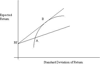
The efficient set is given by the line R_fB. This can be obtained by maximizing the slope of the set of lines passing through the point R_f.

Max s.t. .

The solution is obtained by solving the set of first order conditions:

, for all i = 1,...,N, where g is the Lagrange multiplier.

Substituting Z_k for gX_k, we get

R-R_fi = Q'Z ,
where Q is the variance-covariance matrix of returns, R is the vector of expected returns, and i is the unit vector of length N (i.e. i is an N-vector containing only 1's).

The solution is given by Z =Q^-1(R-R_fi), and

This follows, because Z_k = gX_k, and hence, Z_k = X_k = g.

Short sales allowed, but no riskless lending and borrowing:

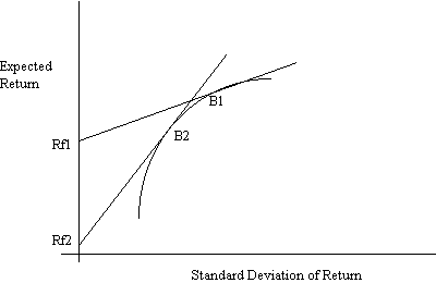
Solve for the tangency portfolio as before with different values for the riskfree rate of return. With R_f = R_f1, we get portfolio B1; with R_f = R_f2, we get portfolio B2. Similarly, we can trace out all other portfolios.

Alternatively, instead of solving the equation Z =Q^-1(R-R_fi) for the particular value of R_f, it is possible to write out the solution in terms of R_f in general:

Z = Q^-1R - (Q^-1)iR_f, where Q^-1R and Q^-1i yield N-vectors.

If we wish to find an efficient portfolio with a given expected return R₀, we just need to find the right value of R_f that will produce an expected return of R₀. This can be done by setting Z'R/Z'i = R₀, and solving for R_f, using the formula above for Z.

This produces a value R_f = R'Q^-1R-R₀[i'Q^-1R]/{R'i-R₀[i'Q^-1R-i'Q^-1i]}.
To confirm, compute the portfolio weights, and check to see if the expected return on the resultant portfolio equals R₀.

Step-by-step calculation of the efficient frontier

First use the return data you have to compute the vector R of expected returns, and Q, the variance-covariance matrix. Q is a matrix containing the variances of the asset returns along the diagonals, and the covariances along the off-diagonals. Thus, if we designate by Q(i,j) the cell representing the intersection of the i-th row and the j-th column, Q(i,j) equals Cov(R_i,R(_j) if i is not equal to j, and equals Var(R_i) if i=j. Obviously, the upper right hand side of the matrix Q is just a reflection of the lower left hand side of Q. Let us take a concrete example, using Excel.

Suppose we have the following data:

The expected return vector, R, is given by

(Note: A vector is a row or column of numbers.)

The variance-covariance matrix, Q, is given by

The numbers, when calculated are:

The next step is to compute the inverse Q^-1. The inverse is also a 3x3 matrix. (For 5 assets, you'd have a 5x5 matrix.)

This is accomplished by using the Excel function MINVERSE. However, in order for the entire inverse to show up, you must highlight a 3x3 area, entire the formula (which in our case is @MINVERSE(Cell Address of Q)), and then press Control, Shift and Enter simultaneously. This will produce Q^-1, the 3x3 inverse of Q. This works out to:

Now, choose any value for the riskfree rate, say 0.05, or 5%. Subtract 0.05 from the expected return vector, R, to create a new vector R-R_fi. In our example, this works out to

Now postmultiply Q^-1 by the vector R-R_fi. Postmultiplication is accomplished as follows:

Multiply the first row of Q^-1 by the vector R-R_fi;
the second row of Q^-1 by the vector R-R_fi;
the third row of Q^-1 by the vector R-R_fi;

(Note: Multiplying two vectors is accomplished by multiplying the first element of the first vector by the first element of the second vector; the second element of the first vector by the second element of the second vector; the third element of the first vector by the third element of the second vector; and adding the three resulting products. In Excel, this can be accomplished by the function @SUMPRODUCT or @MMULT. For @SUMPRODUCT to work, both vectors must be row vectors or both vectors must be column vectors; for @MMULT to work, the first vector must be a row vector and the second vector must be a column vector.)

Alternatively, use @MMULT making sure that you depress Control, Shift and Enter simultaneously, as for MMINVERSE, and that you highlight an area of the appropriate size. In this case, the result of the postmultiplication of Q^-1 by the column vector R-R_fi would be a column vector of length 3.

This gives us three numbers; call these Z1, Z2, and Z3. For our example, the numbers are:

Define three new numbers, X1, X2, and X3, such that X1 = Z1/@sum(Z1,Z2,Z3), Z2 = Z2/@sum(Z1,Z2,Z3), and X3 = Z3/@sum(Z1,Z2,Z3).

For our example, this works out to:

This represents one efficient portfolio. By varying our choice of R_f, we can compute other efficient portfolios. We then compute the expected return and standard deviation of these different portfolios, and then plot them in (E(R), sigma) space as before.

Note that the variance of a portfolio represented by the vector, X, can be computed very simply as (the row vector X) times (Q) times (the column vector X).

Download Excel file with details of the computations presented here. (Click here for information on how to download Excel files.)

Other Links for Portfolio Construction

The Optimization Technology Center has a lot of information on optimization algortihms, among them algorithms for the Portfolio Optimization problem. You can find a demo program with a limited number of stocks here.

Also, check out William Sharpe's website and Prof. Michael Kishinevsky's site.

Go to P.V. Viswanath's Home Page

Go to FIN 652 Home Page