A Primer on Probability
© P.V. Viswanath, 1998,
2000
The material that follows is useful for the analysis of risk and uncertainty as it pertains to the pricing of assets.
Functions
A function is a way of representing a relationship between two variables. In general, a function is represented as a set of pairs of numbers. Thus, the following list of pairs (X, Y) is a function:
| X | Y |
| 1 | 15 |
| 2 | 20 |
| 3 | 25 |
| 4 | 30 |
| 8 | 50 |
| 9 | 55 |
| 12 | 70 |
| 14 | 80 |
In some cases, the relationship can be described by a formula. Thus, if we write Y = 5 + 10X, we are describing two quantities, X and Y, which are represented by several pairs of numbers (Xi, Yi). To obtain the Y value of any given pair, we take the X value, multiply it by 10, and add 5. This also shows that we can consider a function as simply a rule. The list of pairs of numbers above can be described by precisely this function, Y = 5 + 10X.
Graphical Representation of a function
Such a function can also be graphed as a line. Each point on the line represents an (Xi, Yi) pair, with the vertical distance to the X-axis representing the Y-value, and the horizontal distance to the Y-axis representing the X-value. Shown below is a graph of such a function. If we set a equal to 10 and b equal to 5, we have the function described above. Sometimes, we write f(X) instead of Y to indicate that we start with X and perform a sequence of operations on X according to the rule, f, in order to get Y.
Linear and non-linear relationships between two variables
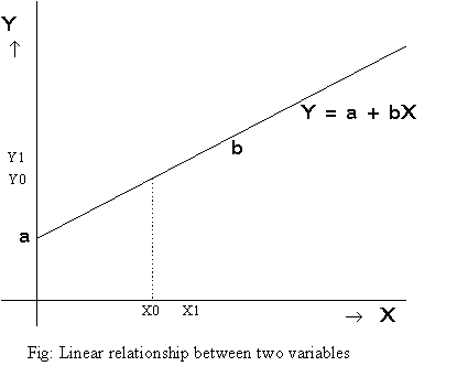
The point where the line intersects the Y-axis is called the
intercept of the graph on the y-axis and equals the number a.
The slope of the line is given by ![]() , where (X0, Y0)
and (X1, Y1) are two points on the line.
, where (X0, Y0)
and (X1, Y1) are two points on the line.
The function graphed above is called a linear function, because the graph of the function is a straight line.
A function can also be non-linear, as in the case below. This function is given by f(X) = 0.1 + 0.2 X + 0.1 X2.
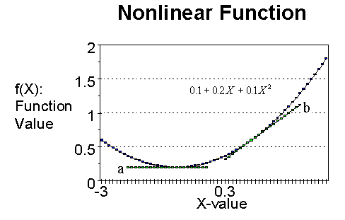
The slope of this function changes from point to point. At a particular point, the slope of this curve is given by the slope of the straight line that is tangential to the curve at that point. Thus, the straight lines marked a and b are tangents to the curve, and their slopes represent the slopes of the curves at the respective points of tangency.
Probability Distributions
A random variable is a variable whose value is subject to uncertainty.
Discrete Distributions:
If X is a random variable and Xi, i=1,..,n are the n possible values it can take with associated (chances of occurring) probabilities pi, i=1,..,n, then the set of numbers (Xi, pi), i=1,..,n is called a probability distribution. Thus, the earnings of Midsoft, Inc. for 1997 could be represented by the following probability distribution.:
| Earnings (Xi) (in million $s) | pi |
| 100 | .2 |
| 20 | .3 |
| -12 | .5 |
We can also consider a probability distribution as a function p(X), where p(Xi) = pi. This function can be represented by means of a graph. The graph for our probability distribution is:
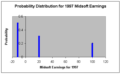
Note that the sum of the pi's is equal to 1, i.e. one of the three scenarios must happen with certainty.
Continuous distributions:
The probability distribution described above is called a discrete distribution because the random variable that it describes takes a finite number of values. It is often convenient to assume that a random variable can take an infinite number of values: for example, the earnings of Midsoft are really not restricted to the values 100, 20 and -12 million. Suppose we allow the earnings to take all possible values, say, between -$20 m. and $200 m., including, for convenience even values in fractions of cents. A probability distribution for this kind of a random variable is called a continuous distribution and differs from the discrete distribution described above in two different ways:
- It is not possible to list the probabilities of all the different values that a continuously distributed variable, such as the earnings, Xi, can take. It is easier to describe the probability distribution by means of a function that describes the relationship between the earnings and the probability. This function can then be graphed in the same way as we graphed the discretely distributed variable above.
- The probability that a continuously distributed random variable takes a single value is close to zero. Thus, the probability that the earnings of Midsoft Corporation are going to be exactly $12 m. is almost zero. Therefore, instead of defining the probability that the random variable takes one particular value or another, we talk about the probability that the random variable will take values within a certain range.
Normal distributions:
For example, a commonly used continuous probability distribution is the normal distribution. This distribution is described by the function
f(X) =  ,
,
where X is a random variable, represents the ratio of the
circumference of a circle to its diameter (approx. 3.14), and the
quantities (expected value) and (standard deviation) represent
different numbers that are different for different random
variables, and X ranges from - ![]() to +
to + ![]() (where
(where ![]() is a very large number). Now, suppose the
return on Trump stock is normally distributed with
is a very large number). Now, suppose the
return on Trump stock is normally distributed with ![]() = 10% and
= 10% and ![]() = 5%; if we plot the probability
distribution, it would look like the graph below:
= 5%; if we plot the probability
distribution, it would look like the graph below:
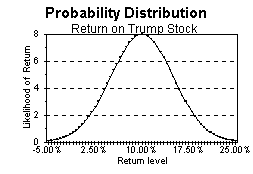
This graph tells us what the likelihood is, of the return being in a small neighborhood of a given level. E.g., the approximate probability that the return will be in a 1% range around the mean 10%, equals the height of the graph at 10% (which is 8) times 1% or 0.01, or 8 x 0.01 = .08 or 8%. However, it only makes sense to ask what the probability is, for a finite range--the probability that the return is exactly equal to 10% is 8 x 0.0 or 0%!
To summarize, we can describe uncertainty about any quantity
by a function called a probability distribution. Like all
(single-valued) functions this, too, is a list of pairs of
numbers. If we have an algebraic description of this function, we
can describe it concisely, as with a normal distribution.
Furthermore, since the only quantities that can be varied in the
description of a normal distribution are ![]() and
and ![]() , different normal
distributions can be characterised by their respective (mean) and
(standard deviation), alone.
, different normal
distributions can be characterised by their respective (mean) and
(standard deviation), alone.
Can we characterize other random variables in a simple way? In general, the most important aspects of any probability distribution are contained in its expected value and standard deviation.
Expected Value or Mean
The expected value, or mean, of a random variable is the
'average' value that the random variable takes. It is defined as ![]()
For example, if we consider the distribution of Midsoft's earnings,
E(X) = .2(100) + .3(20) - .5(12) = 20
The mean of the distribution represents what the earnings of Midsoft would be if we sampled from the distribution over and over -- if the distribution of earnings remained the same over time, the mean would be the average earnings over time. As another example, suppose that the annual return on Trump stock is distributed with a mean of 10%. Then, if we invested in Trump stock time and again, under the same circumstances, we would get 10% on average.
The function E(.) simply represents a weighted average of a quantity, where the weights are the probabilities; hence we can also define the expected value of a function of a random variable:
![]()
Example: Consider two stocks, Duke Energy Corporation (DUK) and Calpine Corporation (CPN). Suppose there are four different scenarios regarding the return on the two stocks for the coming month with the associated probabilities given in the first column. r(duk) and r(cpn) are the returns on the two stocks in the four scenarios.
| Prob. | Scenario | r(duk) | prob x r(duk) | r(cpn) | prob x r(cpn) |
| 0.1 | 1 | 0.10 | .01 | 0.25 | 0.025 |
| 0.3 | 2 | -0.11 | -0.033 | 0.23 | 0.069 |
| 0.4 | 3 | 0.14 | 0.056 | 0.01 | 0.0036 |
| 0.2 | 4 | -0.13 | -0.026 | -0.01 | -0.0010 |
|
E(r) |
0.007 | 0.0966 |
The mean returns are 0.7% per month for Duke and 9.66% per month for Calpine.
Variance
Since E(.) represents a weighted average, the variance is the average squared deviation of a random variable: s2 = E(X - m)2
Consider the variance of the return on a stock, r. If there is a good chance that the return on the stock may be very different from the average return, then those values of the return, r, will contribute a lot to the computation of the expected value of (r-m)2, and the computed value of the variance will be high. The variance thus measures the spread of a probability distribution. The standard deviation is the square root of the variance. The computation of the variance is shown below using the example of the two stocks already described above, Duke Energy and Calpine Corporation.
| Prob. | Scenario | ret(DUK) | Dev. from mean: r(duk)-E(r(duk)) | squared deviation | squared dev. x prob | ret(CPN) | Dev. from mean: r(cpn)-E(r(cpn)) | square | squared dev. x prob. |
| 0.1 | 1 | 0.10 | 0.0930 | 0.0086 | 0.00086 | 0.25 | 0.15340 | 0.02353 | 0.00235 |
| 0.3 | 2 | -0.11 | -0.1170 | 0.0137 | 0.00411 | 0.23 | 0.13340 | 0.01780 | 0.00534 |
| 0.4 | 3 | 0.14 | 0.1330 | 0.0177 | 0.00708 | 0.01 | -0.08760 | 0.00767 | 0.00307 |
| 0.2 | 4 | -0.13 | -0.1370 | 0.0188 | 0.00375 | -0.01 | -0.10160 | 0.01032 | 0.00206 |
| variance | 0.01580 | variance | 0.01283 | ||||||
| std. dev | 0.12570 | std. dev | 0.11325 |
The standard deviation of the returns on Duke Energy is 12.57%, while the standard deviation of returns on Calpine is 11.35%. The probability distribution of Duke Energy and the Calpine Corporation as presented above are clearly not normal; however, to put the quantities that we have just computed into perspective, the expected value and standard deviation of a normally distributed random variable are its parameters m and s.
Sampling as a means of learning about the underlying population distribution
If we know that a random variable's mean value is high, a random draw from the distribution can be expected to be high as well. Similarly, if we know the variance (or standard deviation) is high, we know that realizations deviating a lot from the mean are more likely than otherwise.
But, what if we do not know the actual distribution? Can we infer the true distribution by observing the actual realized values? Obviously, this is an important question because in the real world, we cannot actually observe the true probability distribution. The answer is that we can estimate the true distribution by treating the realized values as a sample from the true distribution. This 'true' or 'actual' distribution that we have just referred to (that presumably truly generates the returns) is called the population distribution; the frequency distribution of observed values in a given sample is called the sample distribution.
For example, if we wanted to know the probability distribution of monthly returns on Duke Energy. If we believed that the future returns on Duke would be drawn from the same distribution as past returns, we could use past data to estimate the distribution of future returns. Thus, suppose we observed the following returns, rTr,t, on Duke for the 30 months from September 1997 to February, 2000:
| Date | return(duk) | Date | return(duk) |
| Feb-00 | -0.1515 | Nov-98 | -0.0242 |
| Jan-00 | 0.1521 | Oct-98 | -0.0227 |
| Dec-99 | -0.0111 | Sep-98 | 0.0611 |
| Nov-99 | -0.0949 | Aug-98 | 0.1023 |
| Oct-99 | 0.0261 | Jul-98 | -0.0359 |
| Sep-99 | -0.0413 | Jun-98 | 0.0282 |
| Aug-99 | 0.0973 | May-98 | 0.0054 |
| Jul-99 | -0.0276 | Apr-98 | -0.0283 |
| Jun-99 | -0.0974 | Mar-98 | 0.0720 |
| May-99 | 0.0878 | Feb-98 | 0.0356 |
| Apr-99 | 0.0217 | Jan-98 | -0.0214 |
| Mar-99 | -0.0363 | Dec-97 | 0.0649 |
| Feb-99 | -0.0714 | Nov-97 | 0.0843 |
| Jan-99 | -0.0351 | Oct-97 | -0.0190 |
| Dec-98 | 0.0240 | Sep-97 | 0.0206 |
We can estimate the population mean by the sample mean, which
is computed as
 , which for our sample yields 0.0055 or 0.55% per month.
The sample variance is computed as
 . In our sample, we get:
| Date | ri | ri
- |
(ri
- |
| Feb-00 | -0.1515 | -0.1570 | 0.024641 |
| Jan-00 | 0.1521 | 0.1466 | 0.021493 |
| Dec-99 | -0.0111 | -0.0166 | 0.000276 |
| Nov-99 | -0.0949 | -0.1004 | 0.010079 |
| Oct-99 | 0.0261 | 0.0206 | 0.000423 |
| Sep-99 | -0.0413 | -0.0468 | 0.002192 |
| Aug-99 | 0.0973 | 0.0918 | 0.00842 |
| Jul-99 | -0.0276 | -0.0331 | 0.001094 |
| Jun-99 | -0.0974 | -0.1029 | 0.010593 |
| May-99 | 0.0878 | 0.0823 | 0.006777 |
| Apr-99 | 0.0217 | 0.0162 | 0.000261 |
| Mar-99 | -0.0363 | -0.0418 | 0.001745 |
| Feb-99 | -0.0714 | -0.0769 | 0.005909 |
| Jan-99 | -0.0351 | -0.0406 | 0.001651 |
| Dec-98 | 0.0240 | 0.0185 | 0.000341 |
| Nov-98 | -0.0242 | -0.0297 | 0.000884 |
| Oct-98 | -0.0227 | -0.0282 | 0.000794 |
| Sep-98 | 0.0611 | 0.0556 | 0.003092 |
| Aug-98 | 0.1023 | 0.0968 | 0.009363 |
| Jul-98 | -0.0359 | -0.0414 | 0.001712 |
| Jun-98 | 0.0282 | 0.0227 | 0.000515 |
| May-98 | 0.0054 | -0.0001 | 2.05E-08 |
| Apr-98 | -0.0283 | -0.0338 | 0.001146 |
| Mar-98 | 0.0720 | 0.0665 | 0.004419 |
| Feb-98 | 0.0356 | 0.0301 | 0.000904 |
| Jan-98 | -0.0214 | -0.0270 | 0.000727 |
| Dec-97 | 0.0649 | 0.0594 | 0.003527 |
| Nov-97 | 0.0843 | 0.0788 | 0.006208 |
| Oct-97 | -0.0190 | -0.0245 | 0.000599 |
| Sep-97 | 0.0206 | 0.0151 | 0.000229 |
| Sample Variance | 0.004483 |
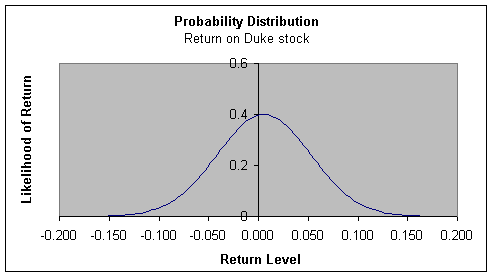
The sample standard deviation becomes 0.0044830.5 or 0.066957 or 6.7% per month. Hence with the given data, we would infer that the return on Duke stock has a probability distribution with mean 0.55% per month and a standard deviation of 6.7%. If we can assume that the stock has a normal distribution, we infer that the probability distribution of the return looks as in the following graph:
Joint Probability Distributions
The uncertainty about a single random variable can be described by its probability distribution. What about a pair of random variables? Their respective probability distributions, of course, provide us with information about them; however when we have more than one variable, we also have to ask how they are related. For example, the height and weight of individuals in the class can be considered random variables. Clearly, though, taller individuals, on average, will tend to weigh more. This information can be captured by what is known as a joint probability distribution.
If we denote height by h and weight by w, here is one example of a joint probability distribution:
| Event | Prob. |
| h |
0.2 |
| h |
0.1 |
| h |
0.05 |
| h > 5'; w |
0.05 |
| h > 5'; 120 < w |
0.1 |
| h > 5'; 150 < w |
0.5 |
From this table, we can see how the two random variables are related. For example, we see by a comparison of rows 1, 2, and 3, that individuals with a height of less than 5' are less likely to weigh above 120 lbs. than below (probabilities of 0.2 and 0.15 respectively).
From this joint probability distribution, we can extract the (marginal) probability distributions for the variables, h and w separately.
Summing over all weight categories, for each h-category, we get the marginal distribution for h:
| Height | Prob. | |
| h |
0.35 | |
| h > 5' | 0.65 |
Similarly, summing over all height categories for each heights for each w-category, we get the marginal distribution for w:
| Weight | Prob. |
| w |
0.25 |
| 150 < w |
0.2 |
| 150 < w |
0.55 |
Two things to be noted:
- A given set of marginal distributions can be associated with different joint distributions.
- We can abbreviate the information about a continuous probability distribution by creating categories.
Covariance
The most important information about the relationship between
two random variables can be extracted from the joint probability
distribution and is given by the covariance: Cov(X,Y) = ![]() x,y =
E[(X-mx)(Y-my)], where mx and my
are the
respective expected values of X and Y.
x,y =
E[(X-mx)(Y-my)], where mx and my
are the
respective expected values of X and Y.
Example: Let us take the case of Duke Energy and Calpine Corporation again. If we posit the following probability distributions, based on the four scenarios, we can compute the covariance.
| Prob. | Scenario | r(duk) | r(cpn) |
| 0.1 | 1 | 0.1000 | 0.2500 |
| 0.3 | 2 | -0.1100 | 0.2300 |
| 0.4 | 3 | 0.1400 | 0.0090 |
| 0.2 | 4 | -0.1300 | -0.0050 |
The covariance is computed by taking the product of the deviations for each variable from its mean return and then computing the weighted average product of deviations.
| Prob. | Scenario | r(duk) | r(cpn) | r(duk)-E(r(duk)) | r(cpn)-E(r(cpn)) | prod of deviations | dev. prod. x prob. |
| 0.1 | 1 | 0.1000 | 0.2500 | 0.0930 | 0.15340 | 0.014266 | 0.001427 |
| 0.3 | 2 | -0.1100 | 0.2300 | -0.1170 | 0.13340 | -0.01561 | -0.00468 |
| 0.4 | 3 | 0.1400 | 0.0090 | 0.1330 | -0.08760 | -0.01165 | -0.00466 |
| 0.2 | 4 | -0.1300 | -0.0050 | -0.1370 | -0.10160 | 0.013919 | 0.002784 |
| covariance | -0.00513 |
The covariance between the returns on Duke and Calpine is, therefore, -0.00513
Whereas the mean and the standard deviation give us information about the probability of a random variable taking on different values, the covariance tells us about the propensity for two random variables to take on combinations of values. For example, suppose Trump and Marriott are both companies in the hotel business; then, we would expect that both stocks would do simultaneously well or simultaneously badly. On the other hand, we would not expect such a scenario with, say, Exxon and Trump. Whether Exxon did well or not, we would not expect Trump to do any differently than if Exxon did not do well. This tendency of two random variables to move or not to move together is measured by covariance.
Recall that E(x) represents the weighted average value of a random variable, x, where the weights are given by the probabilities. Since a transformation of a random variable is also a random variable, (x-mx)(y-my) is also a random variable, which takes different values when x and y take different values.
For example, replace x with the return on Trump stock, and y
with the return on Marriott stock, and let us assume that the
respective mean returns on the two stocks are 5% and 10%. Then,
if the return on Trump stock, denoted rMa, is 3% and
the return on Marriott stock, denoted rMa, is 5%, ![]() takes the value
(0.03-0.05)x(0.05-0.10) or 0.001.
takes the value
(0.03-0.05)x(0.05-0.10) or 0.001.
The covariance between the return on Trump stock and Marriott stock can then be thought of as the expectation or weighted average value of the product of the deviations of the two stock returns from their respective means.
Graphical Interpretation of the Covariance:
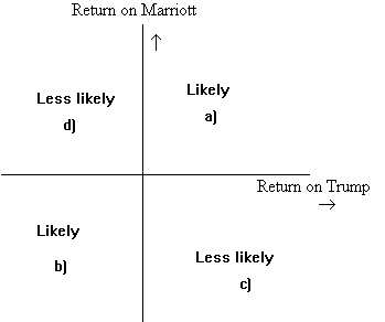
We can think of four classes of outcomes:
- the return on both Marriott and Trump stocks are above their respective means-- rMa > 10% and rTr > 5%;
- the return on both stocks are below their respective means--rMa < 10% and rTr < 5%;
- the return on Trump is above its mean and the return on Marriott is below its mean--rMa < 10% and rTr > 5%; and finally,
- the return on Trump is below its mean and the return on
Marriott is above its mean. For Marriott and Trump, we
would consider scenarios 1) and 2) likely, but not 3) or
4). Now, in quadrants a) and b), the deviations of Trump
and Marriott returns from their means is of the same
sign, and hence the products are positive. In quadrants
c) and d), the products of the deviations are negative.
Hence if quadrants a) and b) are more likely than
quadrants c) and d), the average product of deviations is
likely to be positive, rather than negative.
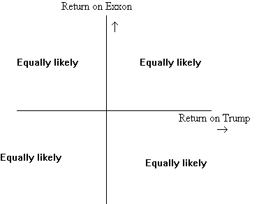
For Trump and Exxon, on the other hand, we might consider all four scenarios equally likely. This means that the positive products of deviations are likely to cancel out against the negative products of deviations, and the average weighted product of deviations will be close to zero.
Sample estimates of the Covariance:
Just as we distinguished between the population and sample marginal distributions, we also distinguish between population and sample joint distributions. Suppose the returns on Trump and Marriott stocks for 10 years are:
| Year | rTr | rMa | Year | rTr | rMa | |
| 81 | 0.06 | 0.17 | 86 | 0.07 | 0.14 | |
| 82 | 0.02 | 0.035 | 87 | 0.08 | 0.18 | |
| 83 | 0.04 | 0.01 | 88 | 0.03 | 0.06 | |
| 84 | -0.01 | 0.045 | 89 | 0.04 | 0.08 | |
| 85 | 0.12 | 0.19 | 90 | 0.05 | 0.09 |
The mean returns can be computed to be 5% and 10% p.a. respectively.
We can compute a sample covariance with the following formula:
 , where the average is computed over the ten months
for which we have data.
| rTr | rMa | Product of deviations | ||
| 0.06 | 0.01 | 0.17 | 0.07 | 0.0007 |
| 0.02 | -0.03 | 0.035 | -0.065 | 0.00195 |
| 0.04 | -0.01 | 0.01 | -0.09 | 0.0009 |
| -0.01 | -0.06 | 0.045 | -0.055 | 0.0033 |
| 0.12 | 0.07 | 0.19 | 0.09 | 0.0063 |
| 0.07 | 0.02 | 0.14 | 0.04 | 0.0008 |
| 0.08 | 0.03 | 0.18 | 0.08 | 0.0024 |
| 0.03 | -0.02 | 0.06 | -0.04 | 0.0008 |
| 0.04 | -0.01 | 0.08 | -0.02 | 0.0002 |
| 0.05 | 0 | 0.09 | -0.01 | 0 |
| Covariance | 0.0019278 |
Correlation Coefficient
It is sometimes difficult to evaluate the degree of
co-dependence of two variables by looking at their covariance,
because its value depends on the units of the standard deviations
of the two variables. We can, however, define another measure, a
normalized covariance, called the correlation coefficient. The
correlation coefficient is defined as ![]() .
.
Going back to our example of a joint population distribution, the standard deviation of the returns on A and B are 0.10 and 0.1151, or 10% and 11.51% respectively, and the covariance is 0.006. Then, the correlation between the returns on A and B is .006/(.1 x .1151) = 0.52.
We can also define a sample correlation coefficient. Thus, for
our sample of returns on Trump and Marriott stock the correlation
is defined as ![]() , or the ratio of the covariance to the product of the standard
deviations. In the case of our sample, this works out to 0.828.
, or the ratio of the covariance to the product of the standard
deviations. In the case of our sample, this works out to 0.828.
The correlation coefficient takes values between -1 and +1. Hence, a value close to +1 indicates a relatively large propensity for the two variables to move together, or covary.
We plot, below, the return on Trump stock against the return on Marriott stock. Consistent with our expectations, all observations fall within quadrants a and b.
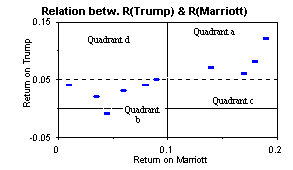
It is clear from what we have seen that knowledge of the actual return on Marriott stock could improve our prediction of the return on Trump stock as well. For example, if we know that the return on Marriott is less than 10%, then we can guess that the return on Trump stock is likely to be less than 5% as well. Such predictions can be made more precise by regression analysis.
Regression Analysis
In regression analysis, we start with the set of points that
we have in the graph above. We then posit a linear relation
between the variable on the y-axis (rTr) and the
variable on the x-axis (rMa), ![]() .
.
However, it is obvious that this relationship is not exact.
Hence, we add an additional term, called the residual that takes
account of this departure from linearity. Symbolically, we write:
![]() .
.
We then choose values for the constants a and b, such that the
importance of the residual or error term, t, is minimized. To
find a unique set of values a and b, we impose, the restriction
that the sum of the squared residuals, ![]() ,
be minimized, so that no individual residual becomes too large.
This defines a unique value for b, which is related to the
covariance:
,
be minimized, so that no individual residual becomes too large.
This defines a unique value for b, which is related to the
covariance:
![]() .
.
We put a hat over the b, to indicate that this is an estimate of the true value of b in the linear relationship between rTr and rMa in the population.
The estimate of a is ![]() . Then, for any given value of rMa,
the predicted value of rTr is simply
. Then, for any given value of rMa,
the predicted value of rTr is simply ![]() .
For our sample, this estimated relationship is shown in the
output from a spreadsheet regression command:
.
For our sample, this estimated relationship is shown in the
output from a spreadsheet regression command:
Constant = 0.0044271 X Coefficient(s) = 0.4557292
R Squared = 0.6995842 Std Err of Coef. = 0.1055852
The return on Trump stock, rTr, is the dependent variable, since we are predicting it, while rMa, the return on Marriott stock, is the independent variable. The Y-variable refers to the dependent variable, and the X-variable refers to the independent variable.
From this output, we see that the estimated regression equation is:
rTr = 0.004427 + 0.45573 rMa.
The standard error of the estimated coefficient, which is
0.1055852 indicates the degree of our confidence in the
coefficient estimate. Just as the given sample is just one of the
many samples that could have been generated by our posited
underlying relationship describing rTr and rMa,
i.e. ![]() , we
can also think of this regression as one of the many
corresponding regressions.
, we
can also think of this regression as one of the many
corresponding regressions.
With this approach, the estimated coefficient for rMa is the estimated mean of the probability distribution of coefficients that such repeated regressions would generate. The standard error, 0.1056, is then like the estimated standard deviation of this probability distribution of coefficients.
This graph shows the actual relationship in the sample between rTr and rMa, and the estimated relationship:
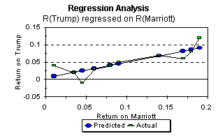
As we saw earlier in our discussion of linear functions, the
estimated intercept â is the predicted value of rTr
if rMa were zero. The estimated coefficient of rMa
in the regression equation, ![]() , is simply the slope of the estimated
linear relationship.
, is simply the slope of the estimated
linear relationship.
For each pair of values, rMa and rTr, in
the sample, we can compute the residual, which is equal to ![]() . In the graph,
this is simply the vertical distance between each actual value
and its predicted value.
. In the graph,
this is simply the vertical distance between each actual value
and its predicted value.