Optimal
Portfolio Construction and Selection
© P.V. Viswanath, 1998,
2000
The idea of risk is intimately tied up with the notion of uncertainty. We will work with the idea that the greater the uncertainty, the greater the risk. A convenient way to represent uncertainty is with a probability distribution. However, a probability distribution has a great deal of information. Our challenge is to distil much of that information into a single number. In order to do that, we will assume that our probability distribution is symmetric, i.e. that the likelihood of deviations below the mean is similar to that of deviations above the mean. This is not unreasonable given the empirical distribution of returns on securities. With this assumption, a good measure of the uncertainty in a probability distribution is the standard deviation (s) of the random variable that is being represented. The standard deviation, intuitively, quantifies the spread of the distribution, i.e. the likelihood of large deviations from the mean. (Strictly speaking, the use of s as a single measure is valid only if the random variable is normally distributed.)
Now, most people dislike uncertainty. Hence, portfolios or strategies that result in high standard deviation of wealth are less preferred compared to those that have low standard deviation. In order to pursue our ultimate goal of locating optimal investment strategies, we need to quantify people's preferences with respect to risk. We will do this by means of a utility function. The utility function that we will employ is the following.
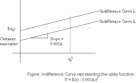
U = E(r) - 0.005As2
In brief, this function measures the utility or desirability of a portfolio or investment strategy by starting with the expected or average return as a base number and subtracting a quantity, which is proportional to the square of the standard deviation of the return on that portfolio or strategy. The square of the standard deviation is known as variance, and the constant of proportionality is 0.005A, where the A is a measure of the risk aversion of the individual, with greater values standing for greater risk aversion.
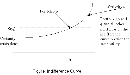
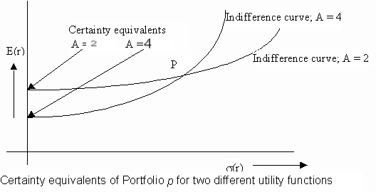
This utility function can be demonstrated graphically by the use of the notion of indifference curves. An indifference curve has the property that the individual is indifferent between all the portfolios that lie on that curve.

We are now ready to use this machinery to investigate the optimal allocation between a risky portfolio and the risk-free asset.
Investing in stocks can be risky. However, this risk can be reduced by allocating part of our investment to risk-free assets.
Definition of a Portfolio: Formally, a portfolio is defined by a set of portfolio weights. Given a list of assets, a portfolio is defined as a set of numbers, wi, such that the sum of the wi equals unity, and wi is the proportion of the wealth in the portfolio allocated to asset i. Using this definition, it is clear that if an asset appears with portfolio weight wi = 0, it does not matter whether it appears in the asset list or not. Hence, we can simply agree to include all assets in the economy in the asset list, and specify portfolios simply by a set of portfolio weights. Under this convention, if there are n assets in the economy, each portfolio is defined as a vector with n components.
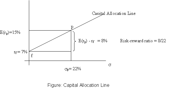
Let C denote the complete portfolio, P the risky portfolio, and f the risk-free asset. Then, if y is the proportion invested in the risky portfolio,
rC = y rP + (1-y) rf
E(rC) = y E(rP) + (1-y) rf, and s C = ys P
From this we can generate the expected return-standard deviation combinations that can be obtained by creating such portfolios. The line joining all such combinations is called the Capital Allocation Line.
What is the optimal amount to invest in the risky asset portfolio if there is one risky portfolio and one riskfree asset?
Suppose the investor likes expected return, but dislikes variance of returns, and his tradeoff between expected return and variance is constant. Then, his utility function can be specified as U = E(r) - 0.005As2, where the parameter A is a measure of his dislike of return variance. We can depict his preferences graphically using indifference curves:
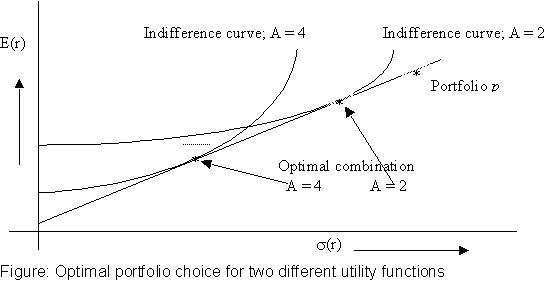
The optimal combination of the risky portfolio, P, and the riskfree asset is given by:

This is obtained by maximizing the utility function subject to the relationships between expected return and standard deviation for the combined portfolio and the expected returns and standard deviations of returns of the risky portfolio and riskfree asset. Click here for a Java program that can be used to compute the portfolio proportions for the optimal combination portfolio. Note that the Risk Tolerance Coefficient in the program equals 200/A. For example, if your A = 10, set the Risk Tolerance equal to 200/10 = 20.
The optimal y* will be higher for investors with lower A:
Under what circumstances would we wish to use the strategy delineated above? Suppose an investor wishes to follow a passive strategy, viz. a strategy that avoids any direct or indirect security analysis. In such as case, his optimal strategy would be to allocate his wealth between a riskfree asset (such as a money market fund, whose exact composition of this portfolio would vary according to his investment horizon) and a broad diversified portfolio (which might, for example, mimic the S&P 500 Index), using the formulas described above. The Capital Allocation line, in this instance, is called the Capital Market Line.
Why might an investor choose a passive strategy? There are two important reasons:
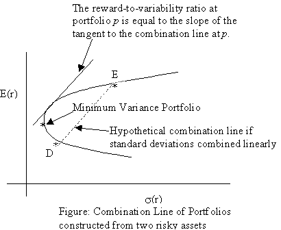
If we wish to construct a portfolio with more than one risky asset, we still use the general utility function approach described above. However, the combination line indicating the expected return-variance combinations that can be obtained with more than one risky asset is no longer linear. We need to consider how portfolio variance changes as we change portfolio proportions. Let us look at the simple case, where there are exactly two risky assets (or portfolios), D and E. Then the expected return and variance of returns is given below:
![]()
![]()
We see below the combination line of the two risky assets, D and E. Note that the portfolio standard deviation is less than the weighted average of the individual standard deviations. Also, the slope of the combination line at any point indicates the reward-to-variability ratio at that point.
The minimum variance portfolio of risky assets D and E is given by the following portfolio proportions:
![]()
The optimal portfolio for an investor with a risk aversion parameter, A, can be represented by the formula:

Graphically, this is the point on the combination line where the slope of the indifference curve is equal to the reward-variability ratio.
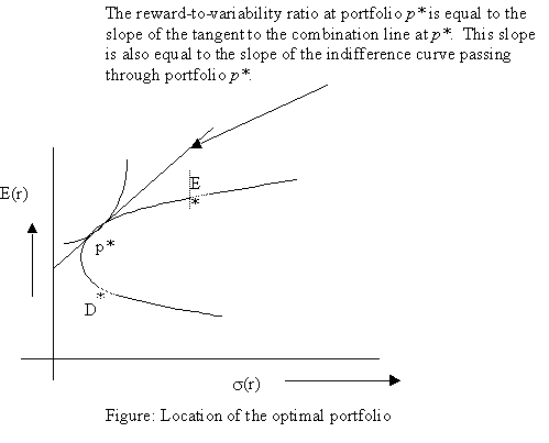
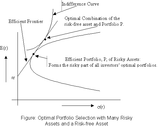
The optimal portfolio choice if there are two risky assets and one riskfree asset can be represented graphically in a similar manner.
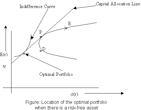
The portfolio proportions for the tangent risky portfolio, P, are:

Note that these weights are independent of the individual investor's risk-aversion. The overall optimal portfolio is then easily computed because this is again a question of choosing the proportion to be invested in a risky asset and a riskfree asset.
Click here for a Java program that can be used to compute the portfolio proportions for the overall portfolio. Note that the Risk Tolerance Coefficient in the program equals 200/A. For example, if your A = 10, set the Risk Tolerance equal to 200/10 = 20.
To see an example of how you can estimate expected returns and variances, and then construct the combination line for two risky assets, go to the spreadsheets on the Webnotes page.
If we have more than two assets, say n assets, then, the expected return is still the weighted average of the expected returns on the component assets, where the weights are the portfolio proportions. The portfolio variance, however, now involves the covariance between every pair of assets.

This can also be represented using the correlation coefficients, rij, as below:

This can be further simplified in terms of the average variance, and the average covariance:
![]()
The greater the number of assets in the portfolio, the closer the portfolio variance gets to the average covariance, and the less it is influenced by the variance of any particular asset. This limit portfolio variance, which cannot be avoided, is called market risk, or nondiversifiable risk, or systematic risk. The risk that can be eliminated from each asset is called idiosyncratic risk, asset-specific risk, diversifiable risk or non-systematic risk. A corollary of this result is that the variance of all well-diversified portfolios are likely to be close to each other.
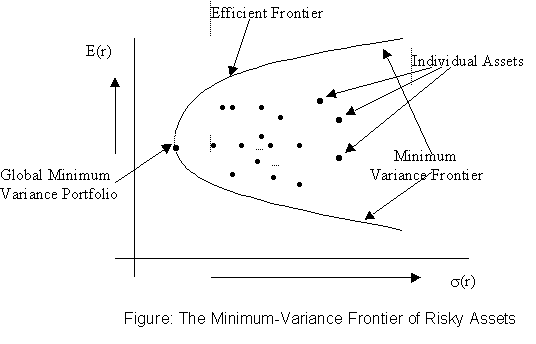
If there are many assets that can be used to form the investor's portfolio, we can construct many combination lines. However, for a given level of risk, an investor will only consider the portfolio with the highest expected return. The set of such portfolios is called the efficient frontier, and is shown below.
