The term
structure of interest rates
ę P.V. Viswanath,
2000
The term structure is the set of interest rates for various terms to maturity embodied in the prices of default-free zero-coupon bonds.
Suppose today’s date is 0. Then, define ri as the short rate that prevails at date i, for the period from date i-1 to i . Hence r1 is the rate today on a one period loan (bond), while r2, r3,... etc; refer to rates on future loans ( one period bonds to be issued in the future). We can also define spot rates yn as the yields to maturity on loans originating today and terminating at time n (zero-coupon bonds issued today and maturing at time n). The term structure of interest rates is given by the set of rates, y1, y2, y3, ...
Example: Suppose today’s date is
January 1, 1980. Consider the prices of the zero coupon bonds in
the table below.
| Maturity date | Pricing date | Price | Notation on Jan. 1, 1980 | Yield |
| 1/1/81 | 1/1/80 | 92.59 | r1 = y1 | 8.00% |
| 1/1/82 | 1/1/80 | 84.17 | y2 | 9.00% |
| 1/1/83 | 1/1/80 | 78.29 | y3 | 8.50% |
| 1/1/82 | 1/1/81 | 90.91 | r2 | 10.00% |
| 1/1/83 | 1/1/82 | 93.46 | r3 | 7.00% |
If, instead of the spot rates, we use the yields to maturity on the most active bonds (not necessarily zero-coupon) of the respective maturities, we get a yield curve.
The term structure and forward rates:
We can also describe the term structure in terms of the set of forward rates. A forward rate is the rate that corresponds to a forward contract. Suppose we enter into an agreement today for a loan commencing at date n-1 and terminating at date n. This is a forward contract. The forward rate, fn, is the rate that corresponds to this agreement.
Note the crucial distinction between a short rate and forward rate: the short rate refers to a rate that is set either today (in the case of r1) or in the future (in the case of all other short rates); the forward rate always refers to a rate that is set today, even though the time period of the loan may be some time in the future. We see that f1 = r1, but fn ≠ rn in general.
We are now ready to see how a term structure can be specified in terms of the forward rates. We do this by presenting the following arbitrage relationship:
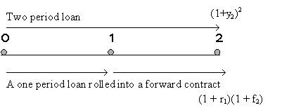
Consider a two period loan. This can be obtained in one of two ways:

The amount to be repaid at the end of the two periods in the two cases would be (1+y2)2 and (1+r1)(1+f2) respectively. Arbitrage will ensure that the two amounts are the same. Hence, we can write 1+f2 = (1+y2)2/(1+r1).
Similarly, it can be shown that 1+fn = (1+yn)n /(1+yn-1)n-1.
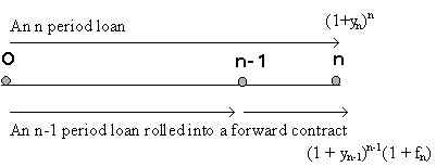
Hence, any sequence of spot rates (yi's) has a corresponding sequence of short rates and forward rates (fi's, where f1 equals r1).
In the same way, any long rate yi can be written as a weighted average of short term rates and forward rates, as follows:
(1+yn) = (1+r1) (1+f2) (1+f3) ... (1+fn).
Hence any theory of the term structure, i.e. about spot rates, makes a corresponding statement about forward rates.
The Liquidity Preference explanation for the Term Structure
Consider a strategy of holding a two period bond versus a strategy of holding one period bonds. The two strategies are not equivalent in a world where future short rates are not known with certainty. Depending upon the horizon of the investor, either strategy can be uncertain.
If we assume that investors have short horizons, then the yield to maturity on a two period bond must be higher than the expected return from rolling over a sequence of one period bonds, since the investor is able to avoid the uncertainty of the price at which the two-period bond can be sold. If we assume that E(ri) is the same for all i, then this implies that the term structure must be upward sloping. However, if investors have longer horizons, then the equilibrium term structure may very well be downward sloping since the longer bond allows the holder to avoid reinvestment risk.
In general, a predominance of short horizon investors (relative to the supply of short-horizon investments) implies that adjusted for expectations of future short rates, the term structure must be upward sloping, while with predominantly long horizon investors, the term structure will be downward sloping, after adjusting for expectations of future short rates.
Consider the investor with a two period horizon:
His terminal dollar return from a 'hold long' strategy is given by (1+y2)2 with zero variance.
The terminal dollar return from a 'hold short' strategy is (1+r1)(1+r2). It's approximate expected value is (1+r1)(1+E(r2)).
If investors with two period horizons predominate, then in order to induce investors to hold the risky one-period bill, it must be true that the expected value of the 'short' strategy is greater than that of the 'long' strategy:
(1+r1)(1+E(r2)) > (1+y2)2 = (1+r1)(1+f2), or E(r2) > f2.
We can implicitly define a liquidity premium, ln, as: fn = E(rn) + ln. Then, it follows that l2 < 0.
If we assume, in addition, that the level of expected future short interest rates is the same as the current short rate, i.e. that E(r2) = r1, then, in this scenario, the term structure must be downward sloping. To see this, note from above, that (1+y2)2 < (1+r1)(1+E(r2)) = (1+r1)2; hence, y2 < y1.
Alternatively, we would say that the expectations-adjusted term structure is downward sloping.
If investors have short horizons, the
inequalities are reversed.
| Investors have short horizons | Investors have long horizons |
| Long bills are risky | Short bills are risky |
| Expectations Adjusted Upward Sloping Term Structure | Expectations Adjusted Downward Sloping Term Structure |
| f2 > E(r2) | f2 < E(r2) |
| Positive liquidity premium | Negative liquidity premium |
Alternative definition of the liquidity premium:
The liquidity premium was defined above as the difference between the forward rate and the expected future spot rate. However, it can also be defined as the additional holding period return over and above the return on the 1-period bond that is required to make investors hold a longer term bond.
For example, the expected holding period return on a 3-yr. bond held for 1 year will be
![]() = r1 + l3.
= r1 + l3.
While the two definitions reflect similar ideas, they are not mathematically equivalent.
The theory does not make any statement about the liquidity premiums; these could be increasing, decreasing or constant across maturities. If we combine different kinds of liquidity premium assumptions with different expectations of futures short rates, we can generate yield curves of varying shapes by using the identity relating spot rates and forward rates: (1+yn) = (1+r1) (1+f2) (1+f3) ... (1+fn).
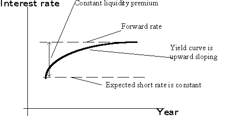
Figure: An upward
sloping yield curve and constant expected short rates
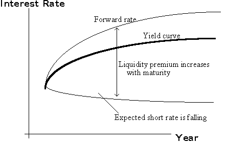
Figure: An upward
sloping yield curve and falling expected short rates
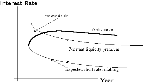
Figure: A humped
yield curve and falling expected short rates
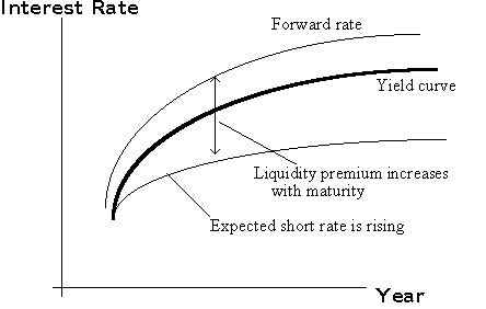
Figure: A rising
yield curve and rising expected short rates
Other Term Structure Theories:
In addition to the theory described above, which is known as the Liquidity Preference Hypothesis, we have two other theories:
The Pure Expectations Hypothesis assumes, effectively, that suppliers of bonds are indifferent between short and long term bonds; or holders of bonds are indifferent between holding short and long term bonds. Then, the forward premium must be zero. In this case, the forward rate simply equals the expected future spot rate.
Hence, (1+y2)2 = (1+r1)(1+f2) = (1+r1)(1+E(r2)).
The yield to maturity on long bonds would be determined solely by current and expected future short rates.
Preferred Habitat/Segmented Markets Hypothesis
This hypothesis focuses on the fact that different segments of the market have different investment needs. For example, insurance companies need to fund long-term liabilities, for which they would prefer long-term bonds. Corporate treasurers may desire short-term bonds to invest funds that they may have temporarily available. This theory suggests that the rates in different maturity segments of the market will depend on the supply and demand for funds in those segments. While there is some truth to this theory, it must be kept in mind that investors in all segments will be willing to hold bonds of longer or shorter maturities provided there is adequate compensation. This links the different maturity segments of the market.
Historical Behavior of the Yield Curve
Historically, term structures seem to be upward sloping more often than not. This suggests that there is a positive liquidity premium embedded in spot yields.
Nevertheless, there is a wide range of yield curve shapes that can be observed in practice. Consequently, it is difficult to actually make any kind of estimate of the term structure of liquidity premiums; for example, one may assume that the liquidity premium is constant over maturities, but this may not be quite true. As a result, the liquidity preference hypothesis can be used mainly as an organizing device to forecast future interest rates given the yield curve and one’s own assumptions regarding investor risk preferences.
Nominal Rates, Inflation and Interest Rate Forecasting:
The nominal interest rate has two components--the real interest rate, and the rate of inflation.
(1+Nominal rate) = (1+Real rate)(1+Inflation rate), or approximately,
Nominal rate = (approx.) Real rate + Inflation rate.
The real rate is compensation for postponing consumption from this period to the next. The inflation rate reflects the change in purchasing power over time and must be added to the real rate because loans are denominated in dollars, and not in units of consumption.
Since the market does not know what the inflation rate will be over the maturity of the bond, it incorporates an estimate of the inflation rate over that period. If, in fact, inflation rates are higher than expected over the period, the realized real rate will turn out to be lower, while if inflation is lower than expected, the reverse will be true.
Example:
Suppose the market requires a real return of 5%
p.a. over the next year, and it also expects inflation over the
next year to be 10%. Then, a one-year zero coupon bond with a
face value of $100 will sell for ![]() .
.
If the actual inflation rate over the next year is 12%, the $100 to be obtained from the bond next year will be equivalent to 100/1.12 = 89.29 of this year’s dollars. The real return, therefore, is 89.29/86.58 - 1 = 3.13% < 5%.
It is easy to see, therefore, that creditors and bondholders benefit from lower inflation, while debtors and bond issuers benefit from higher inflation.
Interest Rate Forecasting
An understanding of inflation is also necessary for interest rate forecasting.
We see from the above discussion that nominal interest rates are already adjusted for expected inflation. Hence, inflation can affect interest rates and thereby bond prices only if market expectations of interest rates change. Interest rates can change, therefore, for two reasons: one, real rates change, and two, expected inflation rates change. Of the two, inflation rates are much more volatile than real rates, and so, more of a change in interest rates is likely to be due to inflation than due to a change in the real rate.
As we have already seen, a rise in bond yields causes a drop in bond prices. Hence, an investor who bets that the market will raise its inflation expectations is betting that interest rates will rise, while one who bets that inflation expectations will fall is betting that nominal rates will fall and that bond prices will rise.
What is important in predicting bond price changes is not whether inflation will increase or decrease but whether it will do so to a greater or less degree than predicted by the market.
Empirically, the shape of the yield curve has also been observed to correlate with the state of the economy. An inverted yield curve where long-term rates are lower than short-term rates is usually associated with future depression.
The term structure theories above were described in terms of the yields on zero coupon bonds. However, most bonds are coupon paying bonds, and we cannot always depend on having the full set of zeros available in order to compute the term structure. How do we obtain the yields on zeros?
A coupon bond can be treated as a portfolio of
zeros. For example, a 2-year 8% bond, paying annual coupons is
equivalent to a 1-year zero with a face value of $80 and a 2-year
zero with a face value of 1080. If such a bond were selling for
$1020, we would write ![]() . In other words, a two-period coupon
bond is a function of the one-period and two-period spot rates.
. In other words, a two-period coupon
bond is a function of the one-period and two-period spot rates.
Define di = 1/(1+yi)i. Then, the price of a 3 period bond paying coupons every period is given by d1C1 + d2C2 + d3C3, where Ci is the cash flow on the bond in period i. Then, if we have the prices of n bonds, we can construct a system of equations:
P1 = d1C11 + d2C12 + d3C13 + ... + e1
P2 = d1C21 + d2C22 + d3C23 + ... + e2
...................................
Pn = d1Cn1 + d2Cn2 + d3Cn3 + ... + en
where Cij is the cash flow in period j on the ith bond, and ei is a residual term to account for any peculiarities of the particular bond, due to special tax or liquidity characteristics.
Regression analysis can be used to estimate
values of d1, d2, d3, and so on,
from which we can generate values for the spot rates.
Go to P.V.
Viswanath's Home Page
Go to FIN 652 Home Page
Go to FIN 351 Home Page