Dr. P.V. Viswanath

pviswanath@pace.edu

Basics of Valuation
©P.V. Viswanath, 2008

• Discounted Cash Flow Valuation
  • Equity Valuation Models
    • Dividend Discount Model
    • FCFE Model
    • FCFF Model
• Relative Valuation

There are two basic approaches to Valuation:

• Discounted Cashflow Valuation - the value of an asset is sought to be obtained directly by valuing the cashflows generated by that asset.
• Relative Valuation - the value of an asset is established relative to other assets.

However, one must recognize that all valuation is ultimately relative, and there are elements of relative valuation in discounted cashflow valuation as well, although this may sometimes be implicit.

Spreadsheet templates applying the different approaches discussed here can be obtained from Prof. Damodaran's website. Some examples of equity valuation using these templates can be found at my classnotes website.

• n = life of the asset
• CF_t = cashflow in period t.
• r = discount rate reflecting the riskiness of the estimated cashflows.

where k_e is the rate of return required by equity investors for the given level of equity risk embodied in the cashflows.

Similarly, we could value the entire firm by taking all cashflows generated by the firm, and discounting them at the weighted average cost of capital: the market value weighted average of the rates of return required by the different security holders of the firm.

Equity valuation models:

• Dividend Discount model:
• FCFE (Free Cash Flow to Equity) Model
• FCFF (Free Cash Flow to the Firm) Model

The Dividend Discount Model simply discounts the dividend per share at the required rate of return. In the general form of the model, the total life of the asset is divided into two parts: an extraordinary growth phase and a stable growth phase.

where

• DPS_t = dividends per share during period t.
• r = required rate of return for equity investors = cost of equity
• P_n = price at the end of year n
• g_n = growth rate forever after year n.

• the length of the high-growth period
• the dividends per share each period during the growth period,
• the rate of return stockholders will demand must be estimated, based on the risk and return model to be used
• the terminal price at the end of the high growth period period

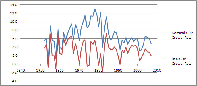
• This rate cannot be greater than the growth rate of the economy, otherwise the firm will become larger than the economy in time; however, the stable growth rate could be smaller than the growth rate of the economy.

Figure: GDP Growth Rate of the US (Source: Bureau of Economic Analysis, http://www.bea.gov/national/index.htm#gdp)

What is the length of the high-growth period?

• the greater the current growth rate in earnings of a firm, relative to the stable growth rate, the longer the high-growth period, although the growth rate may drop off during the period. Thus, a firm that is growing at 40% currently should have a longer high-growth period than one growing at 14%.
• the larger the current size of the firm, the shorter the high-growth period: the larger a firm, the less likely is it to be able to maintain growth.

Expected Dividends during high growth period

• historical growth estimates (use the geometric average of recent years) or
• analyst projections or
• using firm fundamentals

the expected growth rate = retention ratio x return on equity;

Return on equity = ROA + (D/E)[ROA-i(1-t)] where

• ROA = return on assets = EBIT(1-t)/(BV of debt + BV of equity)
• D/E = debt-equity ratio
• i = interest rate on debt
• t = marginal tax rate

• After-tax operating margin = EBIT(1-t)/Sales, and
• Asset Turnover Ratio = Sales/( BV of debt + BV of equity)

Expected Dividends in period t = Expected Earnings in period t x Payout Ratio in period t

We can assume earnings growth to be

• constant during the high-growth phase
• higher during an initial phase, then tapering down to the stable growth rate or
• different during each year depending upon the specifics of the firm.

Finally, we need to estimate the terminal stock price. To do this, we need an estimate of the dividend for the year after the high-growth phase, and the stable growth rate. We should check that the fundamental estimates for the firm during the stable growth period are internally consistent. For example, we have the relation

Growth rate in dividends/retention ratio = ROA + (D/E)[ROA-i(1-t)].

FCFE Model:

FCFE is defined, in general, as

FCFE = Net Income + Depreciation - Capital Spending - D Non-cash Working Capital - Principal Repayments + New Debt Issues.

(Note: Non-cash working capital is used here rather than the broader definition of working capital for two reasons: one, cash is frequently not used for operational reasons; two, cash and cash-like assets and liabilities should be valued differently. Flows from cashlike assets and liabilities should, for obvious reasons, not be discounted at a risky discount rate. Hence cash should be added to the present value of FCFE, in order to get the total equity valuation.

Interest-bearing short-term debt is also cash-like for our purposes, and is better included in financing considerations. Hence, in computing current assets for valuation purposes, we will exclude cash on the assets side and short-term debt (as well as the current portion of long-term debt) on the liabilities side. More information on this can be obtained on Prof. Damodaran's site.

Working Capital usually changes in response to changes in revenues; hence it is best to forecast changes in Non-cash Working Capital in conjunction with revenue forecasts.)

If net capital expenditures (i.e. capital expenditures less depreciation) and working capital are financed at the target debt ratio d , and principal repayments are made from new debt issues, then we have:

FCFE = Net Income - (1-d )(Capital Expenditures - Depreciation) - (1-d )D Non-cash Working Capital, where d is the target debt ratio.

Again, we have a similar valuation formula:

Once again, we can allow for a high growth phase and a stable growth phase.

• First we define the length of the high growth period.
• Using the definition of FCFE, we then estimate FCFE using estimates of Capital Expenditures, depreciation, Working Capital, debt-equity ratio, etc.
• The rate of return required by stockholders is then estimated.
• Finally, the terminal price at the end of the high growth period is estimated based on the estimates of stable growth, the free cash flows to equity and required return after the high growth ends.

We start out with estimating earnings per share, and the growth rate in earnings, as before. We then adjust Net Income by the net capital expenditures, working capital needs, and debt-financing needs. Net capital expenditures and working capital will need to be high for high growth rates to be maintained. Normally, high growth firms are also high risk, and debt is difficult to obtain at reasonable rates. Hence leverage ratios are low for such companies. As growth tapers off, leverage ratios usually go up.

The terminal stock price is estimated using stable period estimates of cash flow, net capital expenditures and working capital needs. Again, consistency is required in the numbers assumed.

The FCFE method will produce different results from the Dividend Discount method if retained earnings are not invested optimally. In particular, if funds are invested in negative NPV projects, the FCFE method could provide higher estimates of value than the Dividend Discount method. On the other hand, if current dividends paid are too high and at unsustainable levels, then securities will have to be issued at high cost to finance the dividends. In this case, the Dividend Discount method will show an ostensibly higher stock value, but one that is not warranted. The key to the value obtained under the FCFE method is in the assumptions that are made regarding capital expenditures and other fundamental variables. The Dividend Discount model is more passive regarding managerial options. If the market for corporate control works well, a higher FCFE method value will eventually lead to a takover, but in the short run, the dividend discount model may not provide a good estimate of value.

FCFF Valuation:

FCFF = Free cash flow to equity + Interest expense (1-t) + Principal Repayments - New Debt Issues + Preferred Dividends.

Alternatively, from a more direct point of view,

FCFF = EBIT(1-t) + Depreciation - Capital Expenditures - D Non-cash Working Capital

The differences between FCFF and FCFE arise from cash flows associated with debt -- interest payments, principal repayments, and new debt issues -- and other non-equity claims such as preferred dividends.

Growth in FCFE versus growth in FCFF. The primary cause of differences in the growth rates in FCFF and the FCFE is the existence of leverage. Leverage increases the growth rate in the FCFE, relative to the growth rate in the FCFF. We can see this from the identity g_EPS = b[ROA + D/E(ROA-i(1-t))]. (b is the retention ratio.) If ROA > i(1-t), then a higher leverage ratio implies a high growth rate in earnings per share and correspondingly in FCFE. On the other hand, the cashflow to the firm is not affected by leverage. The growth rate in EBIT, which effectively determines the growth rate in FCFF will generally be lower and be equal to the product of the retention ratio and the book return on assets.

Again, a high growth phase and a stable growth phase are allowed for. The valuation formula is:

As in the FCFE method, we need the following steps:

• First we define the length of the high growth period.
• We estimate FCFE using estimates of fundamental variables.
• The rate of return required by stockholders is then estimated.
• Finally, the terminal price at the end of the high growth period is estimated based on the estimates of stable growth, the free cash flows to firm and required return after the high growth ends.

This method is easier to apply where cashflows to debt are not smooth and vary over time. At the same time, the firm valuation approach does require information about debt ratios to generate an estimate of the weighted average cost of capital.

The two techniques will provide similar equity valuation numbers if the two conditions are met:

• If consistent growth assumptions are made in the two approaches: this does not mean that the same numerical growth rate is assumed, since the growth rates may differ if leverage is changing.
• If bonds are correctly priced. This follows since the value of equity is obtained from the FCFF valuation of the firm after deducting the value of bonds.

• Firms in Trouble: these firms may have negative cash flows, leading to negative estimated firm values. Estimation of future cash flows is even more difficult.
• Firms in the process of restructuring: these firms may have similar problems. Furthermore, the asset structure of the firm, and the business strategy of the firm may change.
• Cyclical firms: it is necessary to make predictions about the economy as a whole; this may be difficult.
• Firms with Unutilized or underutilized assets: If comparable assets are available that are traded, these values can be used.
• Firms with patents or product options: these real options have to be valued using an option-based analysis, since there may not be any cashflow currently being generated.
• Firms involved in acquisitions: Financial and product market synergies should be taken into account as well.
• Private Firms: risk is difficult to measure; hence it may be difficult to figure out the right discount rate. Market values of assets/securities of the firm may not be easy to obtain.

Estimating Change in Non-Cash Working Capital

This essentially involves utilising existing valuations of 'comparable' assets to price a given asset by working with a common variable such as earnings, cash flows, book value or revenues. Examples:

• Using an industry average P/E ratio to price a firm.
• Using an industry average price to book value ratio.
• Using a price to sales multiple
• Price to cash flows
• Price to dividends
• market value to replacement value (Tobin's Q)

One way to avoid making too many assumptions regarding the comparability of firms is to use equations relating the multiple to fundamentals.

For example, for a stable growth firm, the Gordon Growth models tells us: . Dividing both sides by Earnings gives us a formula for the PE ratio: . This formula allows us to adjust the PE multiple to be used for the firm being evaluated, for differences in its payout ratio, growth rate in dividends, etc. In the same way, formulas can be generated for P/BV (price to book value) ratios and price to sales ratios.

Using multiples depends heavily on assumptions regarding what is comparable. Furthermore, any error that the market has made in valuing the comparables will be carried over the valuation of the firm under consideration.

(based on Damodaran's Corporate Finance, chap. 23.)

Go to Prof. P.V. Viswanath's Home Page

Go to FIN 320 Home Page

Go to FIN 320 Webnotes Page